Linear algebra, particularly Cartesian coordinate systems and vector geometry, is fundamental to CAS. To explain why they are essential to all aspects of CAS, let’s begin with something familiar: a (medical) image:
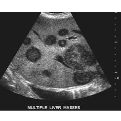
Figure 1:An ultrasound image of a liver containing metastatic cancer growths, image courtesy here, accessed on January 6, 2026.
From Pixels to Positions: Why We Need Coordinates
Consider an US image of a patient’s liver. Displayed on a computer monitor as a {term}`2D’ image of different gray scale, different shades of gray represents different tissues types (often highlighted by tissue boundraries). In Figure 1 for example, a tumour appears as a darker region within the brighter liver parenchyma. But how does one infer the size and location of a tumour based on an image?
Using a digital computer, a grey-scale image is represented as a 2D matrix of numerical values. Each element in this matrix represents a pixel, and the numerical value at each position (pixel) encodes the tissue’s appearance in terms of pixel intensity. For example, Figure 1 is an image of pixels stored as a matrix:
where each represents the intensity value at row and column . Each pixel in an US image is typically represented using a 8-bit of storage (e.g. 1-byte) with the pixel intensity value ranging from 0 to 255, where is pure black and is pure white.
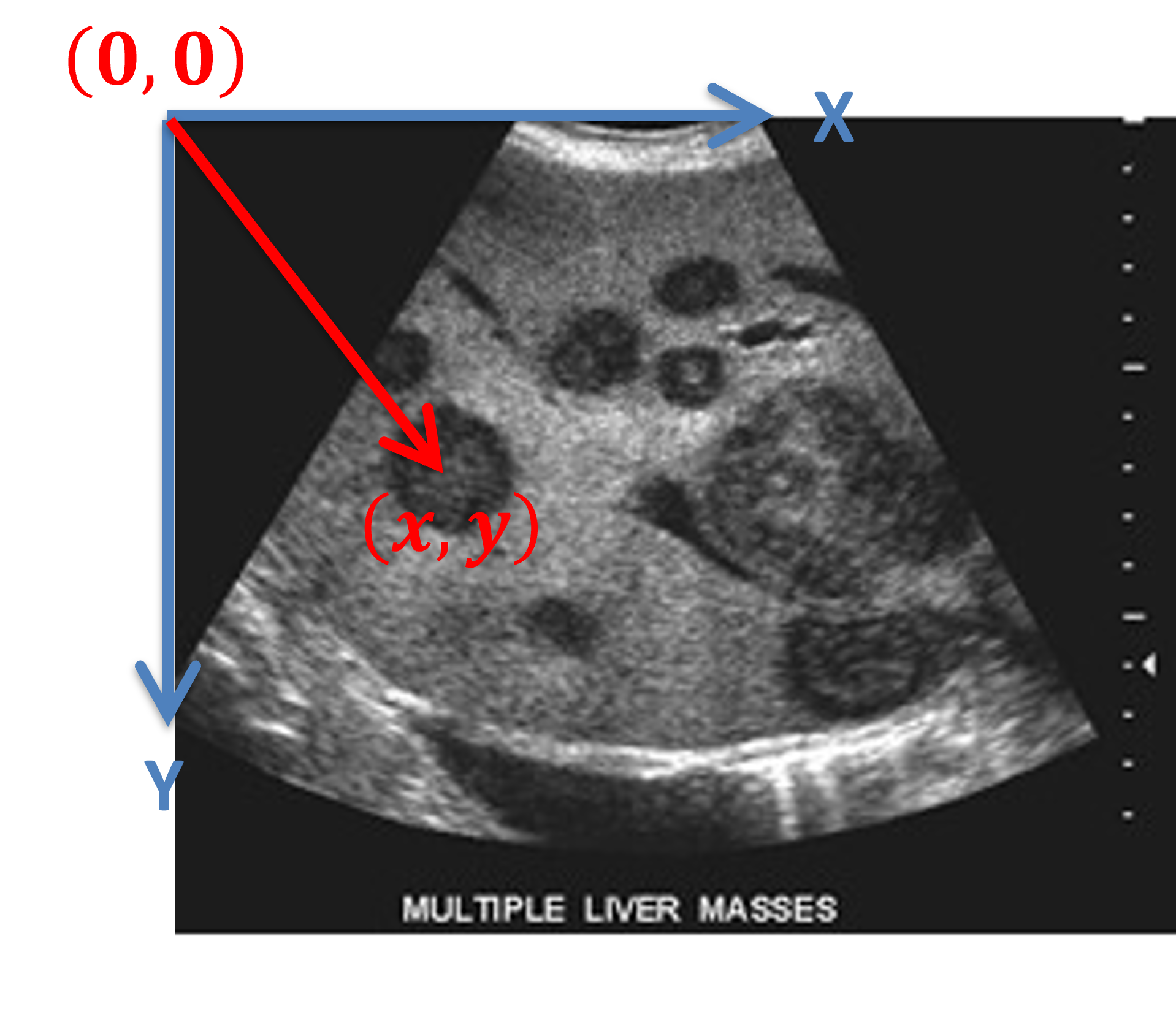
Figure 2:A coordinate system assigned to an US image, where the top-left corner is arbitrary designated as the origin. A pixel at location with an intensity value is thus referred to as , image modified based on the image courtesy here, accessed on January 6, 2026.
That is, each pixel in a 2D image is referred by position, which is also the index to the 2D matrix that is used to store and represent this image in a computer system. The location also represents a vector from the origin of the coordinate system .
The Challenge: From Image Indices to Physical Space
Suppose a radiologist examines this US image and identifies that one of the tumour centre appears at pixel location in the image. The logical questions that follow are:
Where is this location in the patient’s body? This matrix indices does not indicate anything about the physical location of it with respect to the patient.
What about the physical size of the tumour? The 2D matrix, by itself, does not have any information about the physical scale of the image. That is, how do we convert pixel size to a physical unit such as in millimetre?
How do one guide a surgical instrument to this location? Suppose we want to insert a RFA ablation application into this tumour, we need to relate this abstract pixel coordinate system into a physical location that a navigation system can use.
To answer these question requires an understanding of image presentation, coordinate systems, and transformation between coordinate systems. In this regard, a review of linear algebra and vector geometry is needed.
Multi-Channel image and 3D Volumetric Data
While a 2D grey-scale image such as US or X-ray image can be represented by 2D matrix in a digital system, color images and volumetric (i.e. 3D) data requires different representation.
For example, a colour image is typically represented as 3 2D images, each 2D image correspond to a colour channel of red, green, and blue (RGB) primary colours. Conceptually, these 3 2D images can be stacked on top of each other, forming a 2D image but each pixel is a 1D vector of 3 values (i.e. multi-channel).
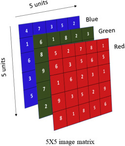
Figure 3:A conceptual representation of a 5x5 RGB colour image, image courtesy here, accessed on January 6, 2026.
A 3D volumetric image data such as CT or MRI are typically displayed, on a 2D monitor, as a series of 2D images:
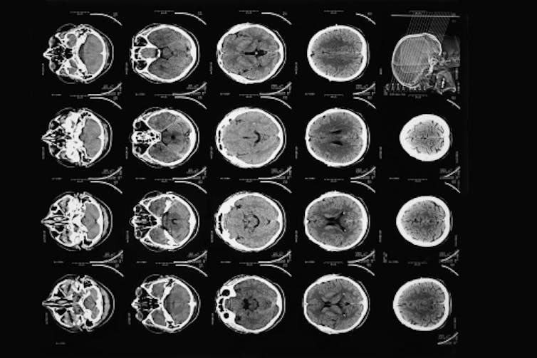
Figure 4:Sequential CT slices displayed as 2D images, image courtesy here, accessed on January 6, 2026.
This was mainly done for historical reasons including the lack of computational power to render these volumetric data in 3D using technique such as Volume rendering.
A volumetric data is presented digitally as 3D array in computer where, conceptually, each 2D slice is assigned a coordinate system and sequential images are stacked in the axis.
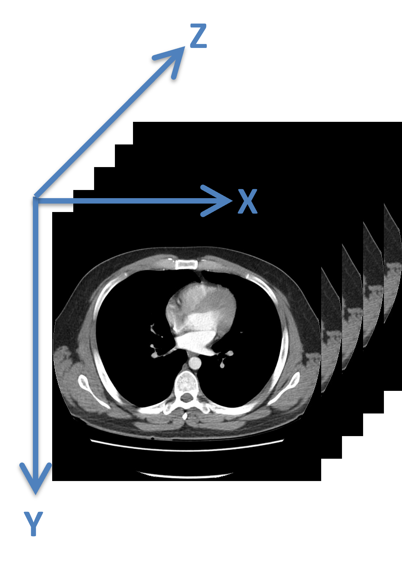
Figure 5:A coordinate system assigned to a 3D volumetric data, where sequential 2D images are assigned a z-coordinate value.
In this regard, each voxel (i.e. a volumetric pixel) is indexed using the notation.
Image Fusion and Augmented Reality Visualization
Image fusion and augmented reality visualization requires the alignment of multiple coordinate systems. This is accomplished via transformation that maps one coordinate system onto another.
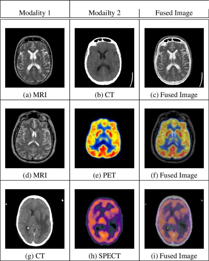
Figure 6:Examples of the common combinations of multimodal medical image fusion (MMIF), image courtesy here, accessed on January 6, 2026.
Categorically, there are three types of transformations:
Rigid transformation
Represented as a transformation matrix that
Rotates, and
Translates one coordinate system onto another.
Similarity transformation
Similar to the rigid translation, but with scaling
Also represented as a transformation matrix
Scaling can be:
Isotropic, same in all 3 directions, or
Anisotropic, different in each direction
Deformable transformation
For the purpose of this course, we focus on only rigid and similarity transformation.
Cartesian Coordinate Systems
The key solution is to establish a Cartesian coordinate system, that specifies each point uniquely by a pair (in 2D) or a triplet (in 3D) of real number called coordinate that in terms allows use to use vector geometry to address these problems.
A Cartesian coordinate system has
Axes, a notation of directions, that intersect at the origin. In most of the scenarios we will encounter in this course, these axes are perpenticular to each other, and
A scale. Each increment, i.e. from to , at a coordinate system may correspond to a physical unit. For example, a pixel in an US image may occupy a physical space of , but a voxel in a CT volume may occupy a physical space of . Often, an anisotropic scaling is needed to match one coordinate system with another.
Vector Geometry: Describing Positions and Transformations
In medical imaging and most of the engineering fields, we use a Right-hand rule (RHR) to define the orientation of the axes with respect to its origin. That is, when extended, if the thumb points at the first (positive x-) axis, and the index finger points at the second (positive y-) axis, then middle finger points to the third (positive z-) axis.

Figure 7:Right-hand rule, image courtesy of Wikimedia Common here, accessed January 9, 2026.
This is the opposite of the left-hand rule, which is more commonly employed in Physics.
Notation for this course:
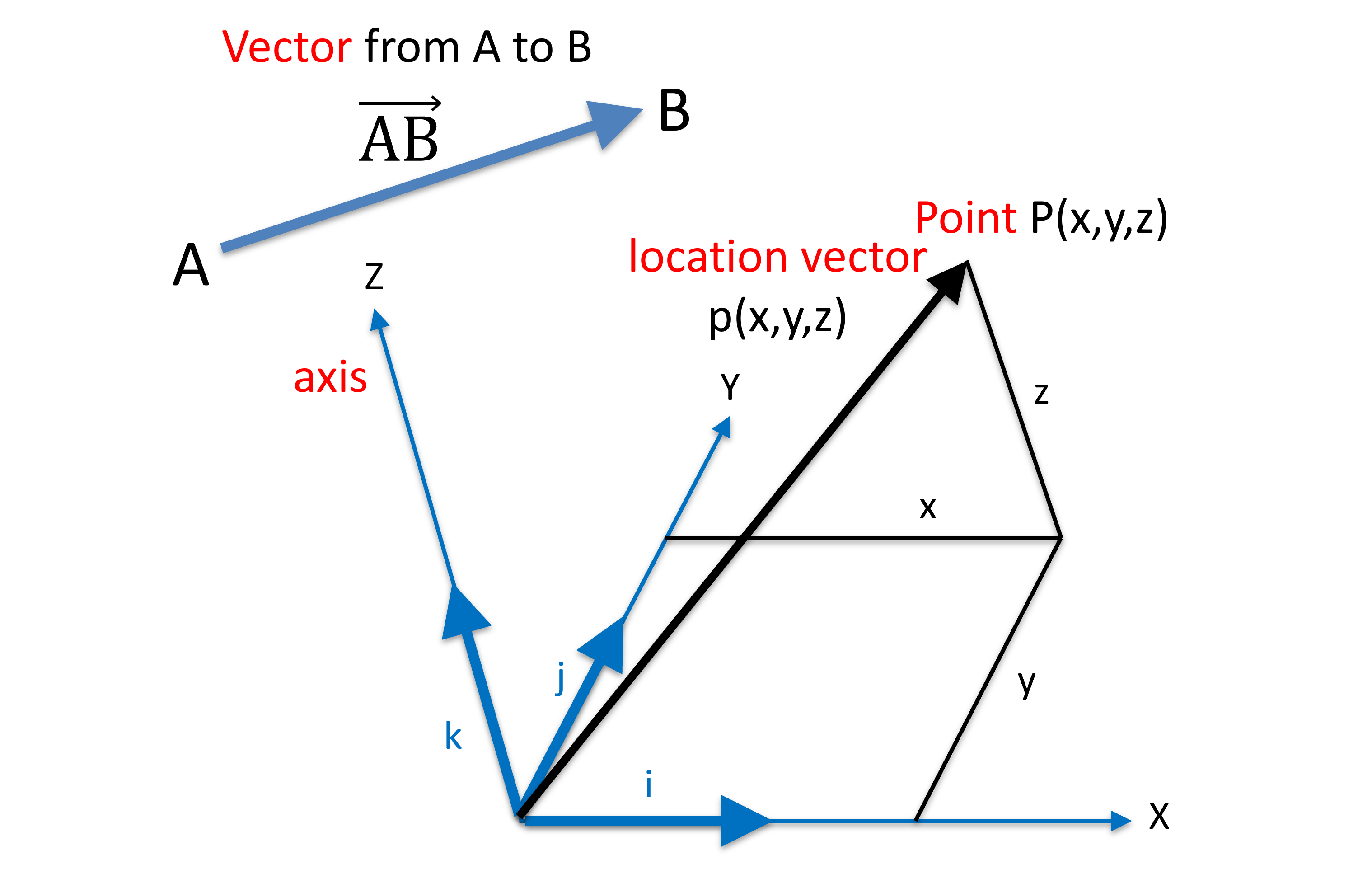
Figure 8:Righthanded Cartesian coordinate system (a.k.a. frame), with orthonormal bases.
We use the following notation:
Points in capital
Vectors and location vectors are usually in lower case, often in italic and/or bold
is for length of a vector or “absolute value”
Sometimes, we omit bold and/or italics
Sometimes, we use location vectors and points interchangeably
Sometimes, we use the same letter and font for x,y,z coordinates and labelling the x,y,z axes
Thus, a location vector p can be expressed by the linear combination of the base vector
and
Skewed Cartesian Frame
Some CT scanners, such as the Toshiba Asteion 4, has the ability to performed tilted scan. The intended use is, as an example, reduce X-ray radiation dose to patient’s eye lenses.
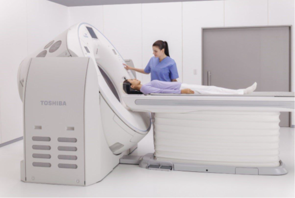
Figure 9:A Tilted Computed Tomography (CT) machine, aimed to reduce X-ray dose to eye lenses, image courtesy of Prof. Gabor Fichtinger at Queen’s University, Canada
In this scenario, the base vectors are no longer pair-wise orthogonal, however, a point P or location vector can still be represented by the linear combination of the base vector
But the length of the vector is no longer the square root of the sums of the squared coordinates:
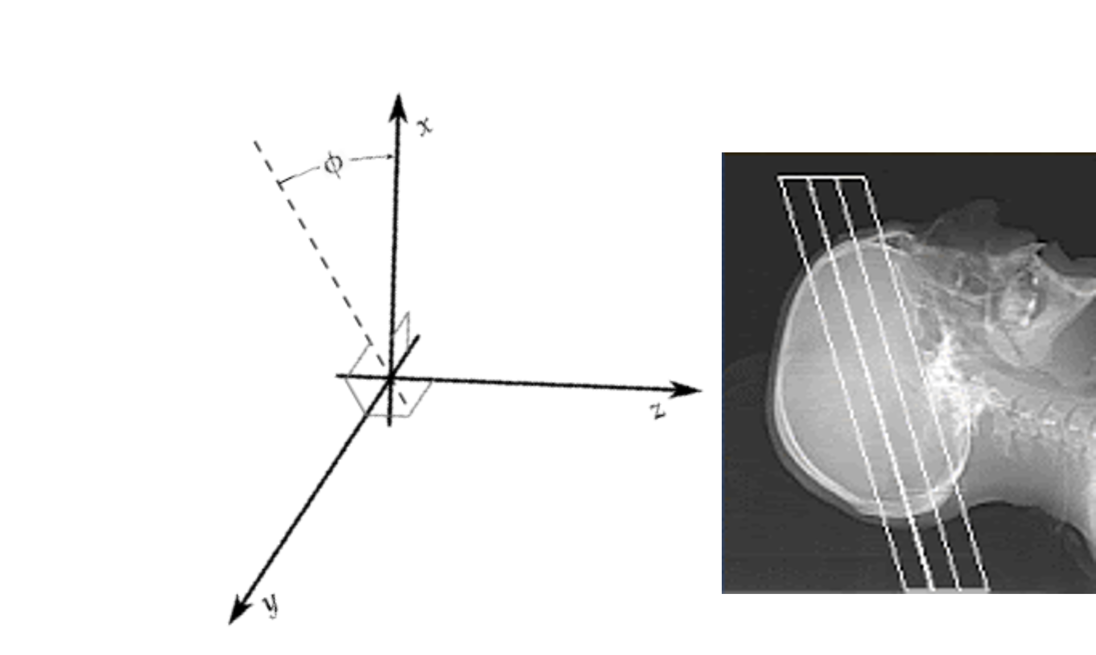
Figure 10:A Tilted Computed Tomography (CT) image volume, image courtesy of Prof. Gabor Fichtinger at Queen’s University, Canada
Polar Frames
For mathematical convenience, polar frames are often be used to represent coordinate systems.
Spherical Coordinate System
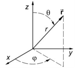
Figure 11:The spherical coordinate system, where the vector is denoted by 2 angles and the length of the vector, image courtesy of Prof. Gabor Fichtinger at Queen’s University, Canada.
A vector with a vector length is denoted by its length and two angles from - and -axes:
A use case for spherical coordinate system is the Lars Leksell frame:
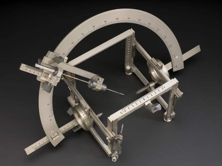
Figure 12:A version of the Leksell Stereotactic frame with angular marking, image courtesy here, accessed January 8, 2026.
commonly used for neurosurgery for inserting a (biopsy/electro) needle:
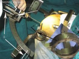
Figure 13:A Leksell frame used in OR, image courtesy of Prof. Gabor Fichtinger at Queen’s University, Canada
Because needle is more intuitively represented as a vector (i.e. a point with direction), the use of the spherical coordinate system is more mathematically convenient.
Cylyndrical Coordinate System
The cylindrical coordinate system is used to describe a point on the surface of a cylinder, where a point is represented by a lenth (radius of the cylinder), an angle , and the height :
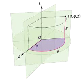
Figure 14:The cylindrical coordinate system, where the vector is denoted by 1 angle and a length, and the height, image courtesy of Prof. Gabor Fichtinger at Queen’s University, Canada.
One use of the cylindrical coordinate system is the intracavity robot, where an, as an example, a transrectal ultrasound (TRUS) is use in surgery.
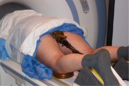
Figure 15:A transrectal ultrasound used an MRI suite, image courtesy of Prof. Gabor Fichtinger at Queen’s University, Canada
Because the TRUS is a cylindrical object, it is more convenient to define a points on its surface (and thereby a direction) using the cylindrical coordinate system.

Figure 16:A transrectal ultrasound transducer, image courtesy of Prof. Gabor Fichtinger at Queen’s University, Canada
- Ibrahim, Sa. I., El-Tawel, Gh. S., & Makhlouf, M. A. (2023). Brain image fusion using the parameter adaptive-pulse coupled neural network (PA-PCNN) and non-subsampled contourlet transform (NSCT). Multimedia Tools and Applications, 83(9), 27379–27409. 10.1007/s11042-023-16515-2