In this section, geometrical primitives including
point,
vector,
line,
plane,
spheres, and
ellipsoids
and their mathematical operations, are introduced.
Point
In geometry, a point is an abstract idealization of an exact position, with no size or mass, in space. For this ource, this space is the [Cartesian space]Cartesian coordinate system, thus the position of a point is its coordinates.
Visualization
Visualization using computer graphics is a very helpful way to
understand the geometrical relationships, and
validation the results of a numerical solution of an algorithm.
Here, we introduce Visualization Toolkit, or VTK.
The example below depicts a single point as a sphere in a 3D Cartesian coordinate system. The full source code is here.
Step 1: Import External Libraries
Working in Python, we need to import all the neessary functions and external libraries first. This includes numpy and vtk filters:
import math
import numpy as np

# noinspection PyUnresolvedReferences
import vtkmodules.vtkInteractionStyle
# noinspection PyUnresolvedReferences
import vtkmodules.vtkRenderingOpenGL2
from vtkmodules.vtkCommonColor import vtkNamedColors
from vtkmodules.vtkCommonTransforms import vtkTransform
from vtkmodules.vtkFiltersSources import vtkSphereSource
from vtkmodules.vtkRenderingAnnotation import vtkAxesActor
from vtkmodules.vtkRenderingCore import (
    vtkActor,
    vtkPolyDataMapper,
    vtkRenderWindow,
    vtkRenderWindowInteractor,
    vtkRenderer
)
Step 2: Rendering Pipeline
We need to set up a rendering pipeline. In VTK, this includes:
A vtkRenderWindow is a window in a graphical user interface (GUI) where a renderer draw their images,
A vtkRenderer is an object that controls the rendering process of objects, and
A vtkRenderWindowInteractor provides an interaction mechanism better users (i.e. mouse inputs) and the render window
# Visualization Pipeline

# a renderer and render window
ren = vtkRenderer()
renWin = vtkRenderWindow()
renWin.SetWindowName('AISE 4025: point and axes')
renWin.SetSize( 640, 480 )
renWin.AddRenderer( ren )

# an interactor
iren = vtkRenderWindowInteractor()
iren.SetRenderWindow( renWin )
Step 3: Geometrical Primitives
A geometrical primitives such as a point and a line is created by
a source, i.e. its mathematical description
a mapper, an object that translates the source to,
an actor, the final object that is to be rendered in the renderer. For geometrical objects, they are typically a set of connected triangles
colors = vtkNamedColors()

# Create a sphere to represent a point
point = np.array([0, 5, 0])         # position of a point

# use a sphere with a finite size to visualiza a point, since a point, by definition, has no size
sphereSource = vtkSphereSource()
sphereSource.SetCenter( point.tolist() )
sphereSource.SetRadius( 0.5 )       # an arbitrary size

# create a mapper
sphereMapper = vtkPolyDataMapper()
sphereMapper.SetInputConnection( sphereSource.GetOutputPort() )

# create an actor
sphereActor = vtkActor()
sphereActor.SetMapper( sphereMapper )
sphereActor.GetProperty().SetColor( colors.GetColor3d('Red') )
We can add a 3D axes to help us orient
# add an 3D Axes
axes = vtkAxesActor()
axes.SetTotalLength(10,10,10)
axes.AxisLabelsOff()

# properties of the axes labels can be set as follows
# this sets the x axis label to red
axes.GetXAxisCaptionActor2D().GetCaptionTextProperty().SetColor(colors.GetColor3d('Red'));
axes.GetYAxisCaptionActor2D().GetCaptionTextProperty().SetColor(colors.GetColor3d('Green'));
axes.GetZAxisCaptionActor2D().GetCaptionTextProperty().SetColor(colors.GetColor3d('Blue'));
Step 4: Rendering
Add all actors to the renderer so the renderer knows what to draw.
# Add the actors to the scene
ren.AddActor( sphereActor )
ren.AddActor( axes )
ren.SetBackground( colors.GetColor3d( 'MidnightBlue') ) # the color can be specified as a name
ren.SetBackground( .1, .2, .4 )                         # or as RGB
ren.SetBackground( 1, 1, 1 )                            # this is white
ren.ResetCamera()
renWin.Render()
iren.Start()In this particular example, the point is loccated at , i.e. on the -axis. We draw a red sphere at that location, where each of the -, -, and -axis is shown as red, green, blue lines with arrow.
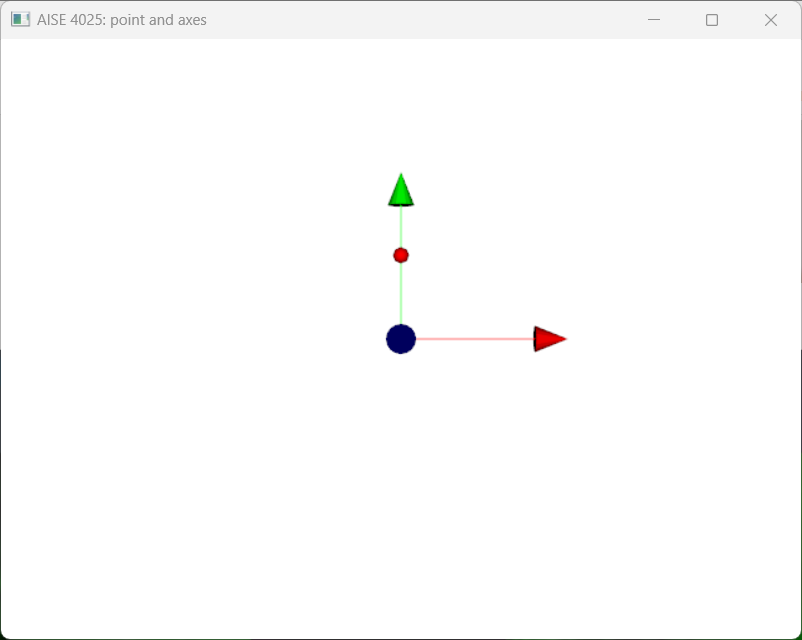
Figure 1:A point visualized as a red sphere.
Draw onto the render window and start the user interaction.
Vector and Unit Vector
While a point specifies the position of an object in the {wiki:Cartesian_coordinate_system}, a vector is used to specify the orientation of an object. As such, a vector is not fixed on the {wiki:Cartesian_coordinate_system} at a given location.
It is often useful to think of the position of a point as a vector, originated from the origin to the point, instead.
For mathmatical convenience, a unit vector, a vector of length 1, is often used to represent the orientation.
A unit vector is a vector with length one:
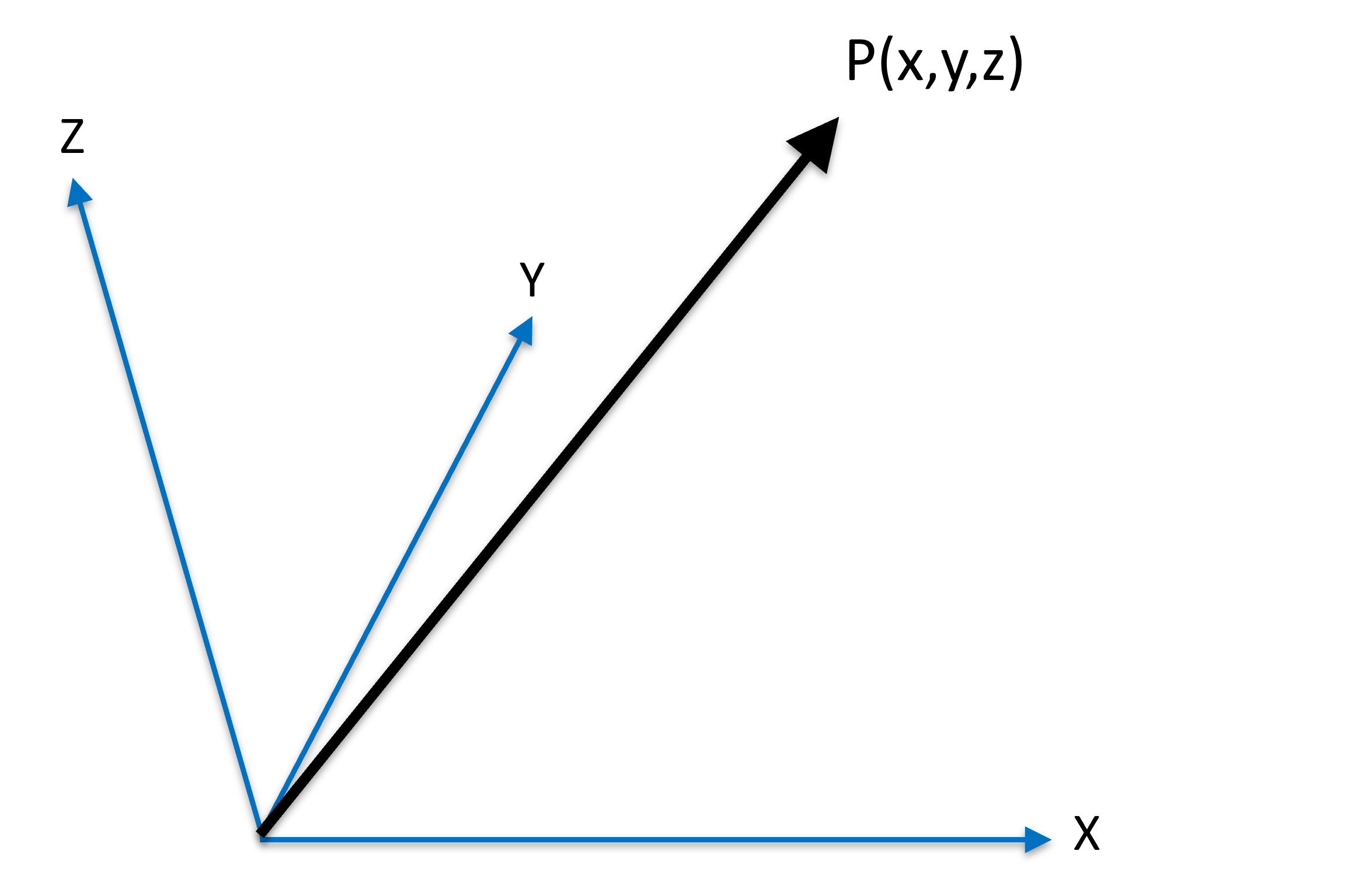
Figure 2:A unit vector originated from origin to location .
That is,
"""
@author: Prof. Elvis C. S. Chen

January 8, 2026
"""

import math
import numpy as np
import numpy.matlib

p = np.array([ 1, 0, 0 ])      # This is a ROW vector
p = p.reshape(-1, 1)           # this is a COLUMN vector
p = np.array([ [0],[1],[0] ])  # alternative
print("The 3x1 colume vector:\n", p)
print(p.shape)
print("The length, or norm, of this vector is: ", np.linalg.norm(p))       # Length of the vector can be calculated using numpy
The 3x1 colume vector:
[[0]
[1]
[0]]
(3, 1)
The length, or norm, of this vector is: 1.0
Scaling of a Vector
A vector can be scaled up (i.e. lengthening) or down (i.e. shortening) by a scalar factor
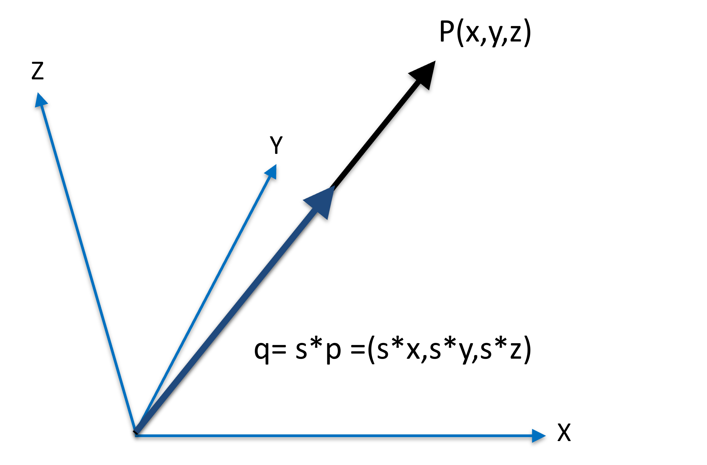
Figure 3:A vector beins scaled as .
If
, the vector is being lengthened,
, the vector is being shortened,
, nothing happens,
, something is probably wrong,
, the orientation of the vector is changed, in addition to being lengthened/shortened.
# demonstration of scaling of a vector
s = 0.75 # Scaling the vector by a factor of 0.75
q = s * p
print("The original vector p is\n", p, "\nand the scaling factor is:", s, "\n")
print("q is the scaled vector of p: \n", q, "\nwith the norm of the vector being:", np.linalg.norm(q))
The original vector p is
[[0]
[1]
[0]]
and the scaling factor is: 0.75
q is the scaled vector of p:
[[0. ]
[0.75]
[0. ]]
with the norm of the vector being: 0.75
Obviously, scaling of a vector changes its length accordingly.
Normalizing a Vector
Normalizing a vector meaning to change the vector length to 1:
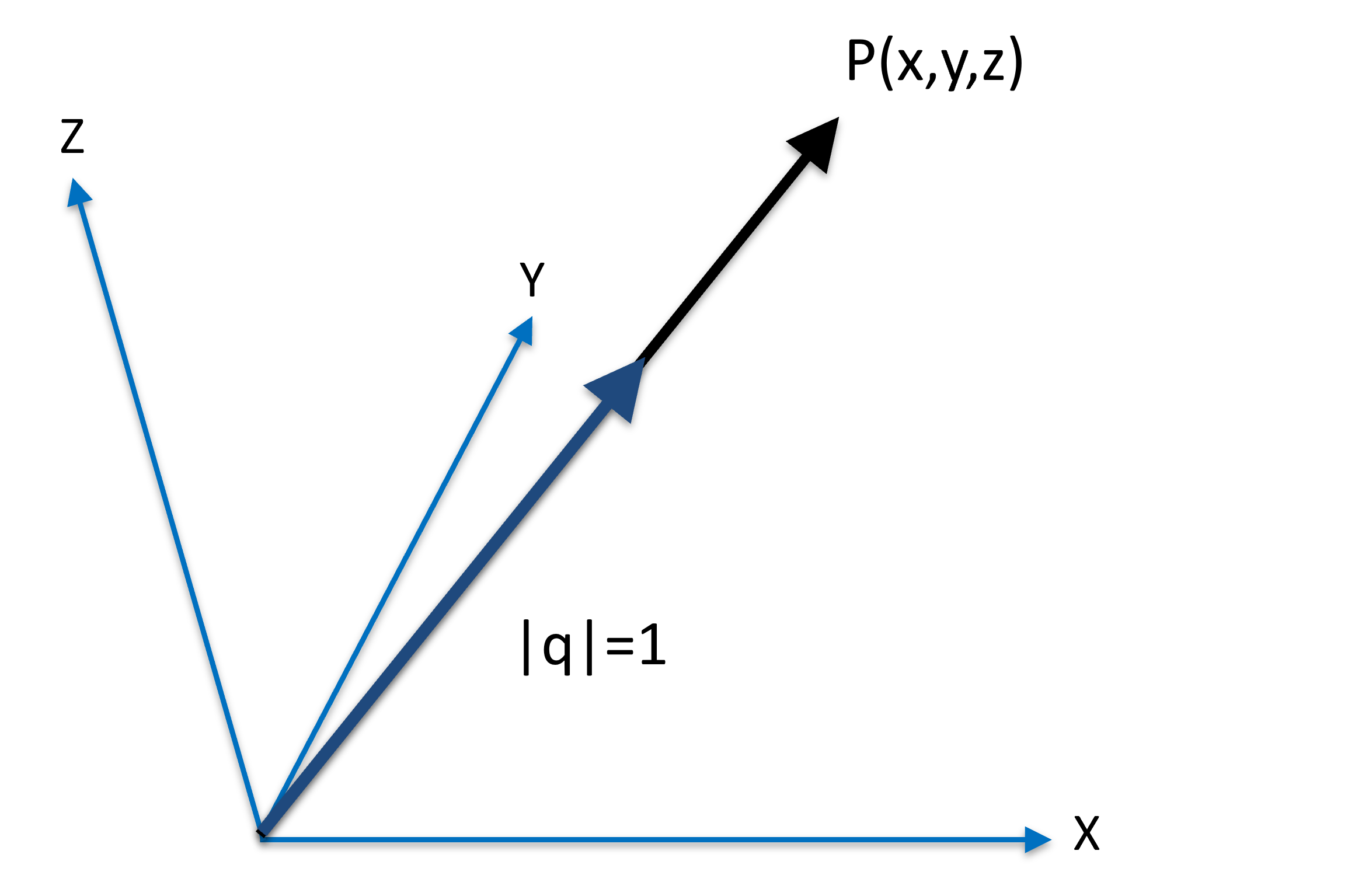
Figure 4:A vector beins normalized as as .
In Figure 4, the vector is the normalized version of , as the length of is 1; both and are originated from the origin, pointing in the same direction.
p = np.array([ 3, 4, 5 ])      # This is a ROW vector
p = p.reshape(-1, 1)           # this is a COLUMN vector

q = p/np.linalg.norm(p)
print("The original vector p\n", p, "\nhas a length of", np.linalg.norm(p), "\n")
print("The normalizes vesion q\n", q, "\nhas a length of", np.linalg.norm(q), "\n")
The original vector p
[[3]
[4]
[5]]
has a length of 7.0710678118654755
The normalizes vesion q
[[0.42426407]
[0.56568542]
[0.70710678]]
has a length of 0.9999999999999999
Sum of Vectors
Just like scalars, vectors can be added and substracted. Adding two vectors means that you contatenate the end of one vector to the origin of another:
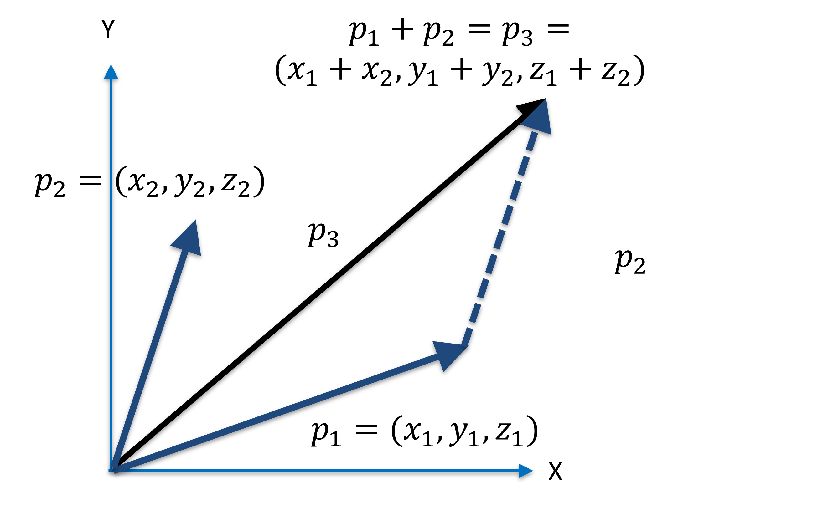
Figure 5:Sum of vectors is the same as concatenating the vectors.
In Figure 5, the vector is the sum of and :
p1 = np.array([ 1, 2, 3 ])
p2 = np.array([ 4, 5, 6 ])
p1 = p1.reshape(-1,1)
p2 = p2.reshape(-1,1)

p3 = p1 + p2

print("the sum of vector 1\n", p1, "\nand vector 2\n", p2, "\nis\n", p3)
the sum of vector 1
[[1]
[2]
[3]]
and vector 2
[[4]
[5]
[6]]
is
[[5]
[7]
[9]]
For visualization, consult the following tutorial.
Distance between two Points
The distance between two points and is the length of the vector (or ):
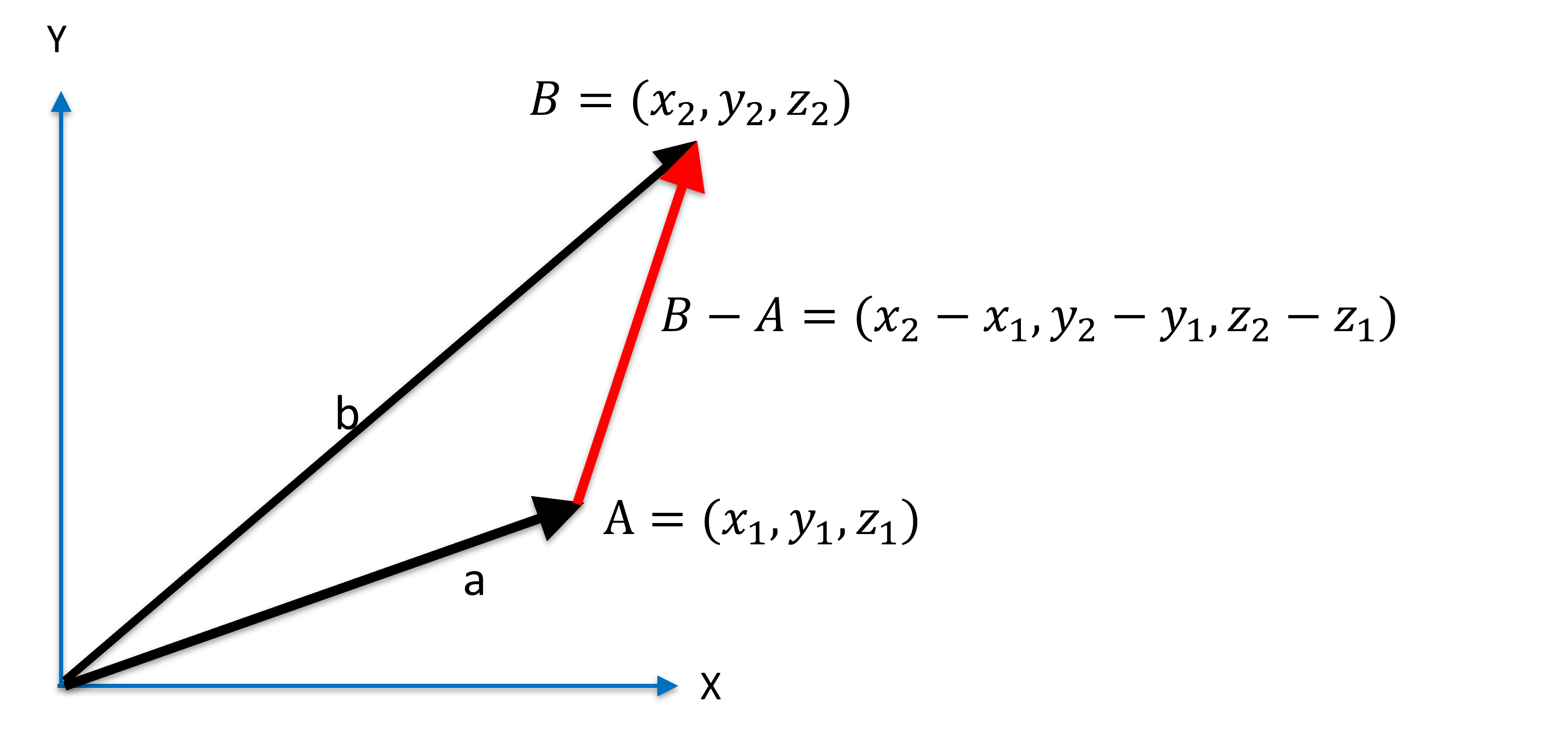
Figure 6:Distance between two points.
print(np.linalg.norm(p2-p1))
print(np.linalg.norm(p1-p2))
5.196152422706632
5.196152422706632
Cross Product between two Vectors
Cross product between vectors and results in a third vector that is perpendicular to both and , with the direction of vector that obeys the RHR. That is, if the right-hand index finger points in the direction of the vector , and the right-hand middle finger points in the direction of the vector , then the thumb points to the direction of . Cross product is denoted by the symbol .

Figure 7:Right-hand rule, image courtesy of Wikimedia Commons here, accessed January 9, 2026.
This directionality implies : cross product is not communitive. In fact, the cross product is anticommutative:
Cross product is distributive, however:
The cross product between and can be expressed as the formal determinant:
As such, the magnitude of the resulting vector is:
where is the angle between vectors and .
Using this property, the cross product can be used to check if two vectors are parallel or antiparallel: in these scenarios, the cross product results in a zero vector with a length of 0:
a = np.array([ 1, 0, 0 ])     # this is a row vector
b = np.array([ 1, 0, 0 ])
a = a.reshape(-1,1)           # this is now a column vector
b = b.reshape(-1,1)

c = np.cross(a, b, axis=0)
print("The cross prouct is:\n",c)
print("with the length being:", np.linalg.norm(c))

# what does this line do?
print(np.asin( np.linalg.norm(c) / ((np.linalg.norm(a))*(np.linalg.norm(b))) ) * 180.0 / np.pi )
The cross prouct is:
[[0]
[0]
[0]]
with the length being: 0.0
0.0
You should experiment with the above code, by using different values for and , and convince yourself that:
Indeed the cross product vector is perpendicular with both and , and
Indeed you can infer the angle between and
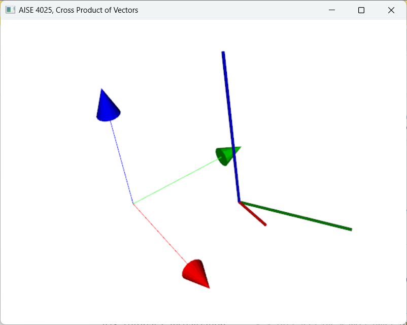
Figure 8:The cross product between the red vector with the green vector produces a blue vector that is perpendicular to both the red and green vectors.
For visualization, consult the following tutorial.
Orthonormal Basis from Three Points
One utility of cross product often encountered in CAS is to define a unique Cartesian coordinate system based on 3 points.
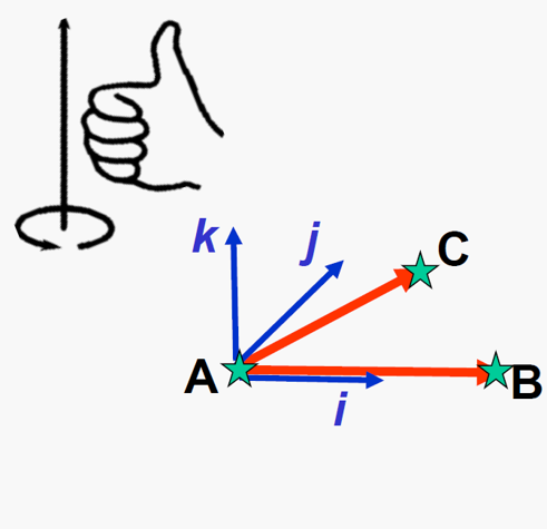
Figure 9:A orthonormal basis of can be created from 3 points , , and using vector subtraction and cross product, image courtesy of Prof. Gabor Fichtinger at Queen’s University, Canada.
The axes of the Orthonormal Basis
Given three points , , and , the process of creating a orthonormal basis while keeping the RHR are:
Create the axis by ,
Create the axis by , and
Create the axis by
Normalize each axis
Note the order of which axis is computed, and try to understand why by visualizing. Normalization of the axes should be performed before taking the cross product to ensure numerical stability.
A = np.array([ 0, 0, 0 ])     # this is a row vector
B = np.array([ 2, 0, 0 ])
C = np.array([ 3, 4, 0 ])
A = A.reshape(-1,1)           # this is now a column vector
B = B.reshape(-1,1)
C = C.reshape(-1,1)

i = (B-A)/np.linalg.norm(B-A)

k = np.cross(i, (C-A)/np.linalg.norm(C-A), axis=0)
k = k/np.linalg.norm(k)

j = np.cross(k, i, axis=0)

print("Basis axis-i, i.e., x:\n", i)
print("Basis axis-j, i.e., y:\n", j)
print("Basis axis-k, i.e., z:\n", k)
Basis axis-i, i.e., x:
[[1.]
[0.]
[0.]]
Basis axis-j, i.e., y:
[[0.]
[1.]
[0.]]
Basis axis-k, i.e., z:
[[0.]
[0.]
[1.]]
The Origin of the Orthonormal Basis
As a Cartesian coordinate system has an origin, i.e. a common point where all directional axes intersect at, we must define one.
There are two practical choices:
Desginate one of the three point as the origin, and associate all axes with it, or
use the Center of Gravity (COG), i.e. the centroid of the 3 points.
Mathematically, the origin of the newly define Cartesian coordinate system can be anywhere. The COG is a reasonable choice, calculated as the unweighted average of the points:
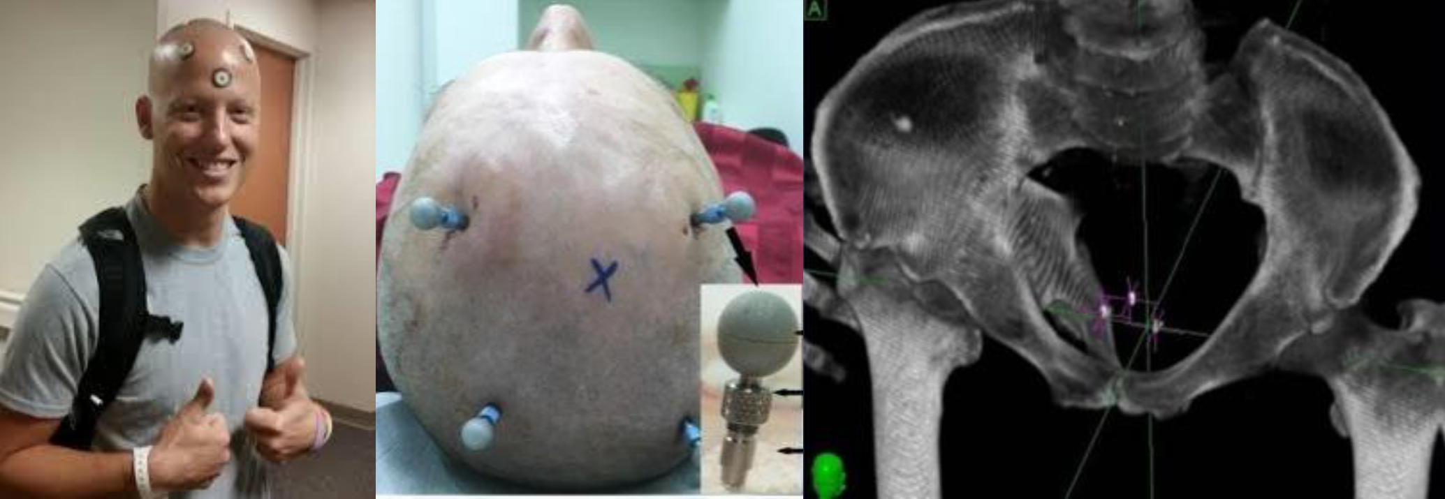
Figure 10:Use case for defining a reference frame including tracking objects, image courtesy of Prof. Gabor Fichtinger at Queen’s University, Canada.
Defining a reference Cartesian coordinate system from three points is used in many techniques in CAS; mainly for tracking objects.
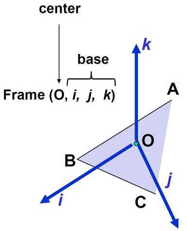
Figure 11:A reference Cartesian frame defined from points , CO$ is located at the Centre of Gravity, image courtesy of Prof. Gabor Fichtinger at Queen’s University, Canada.
For visualization, consult the following tutorial.
Area of a Triangle
Visualization in CAS uses techniques from computer graphics including surface wire-frame or Volume rendering. The most common representation of an object with complex geometry is to represent it as a set of connected triangles via a process called polygon triangulation. In this regard, area of a triangle, and the summation of connected triangles, yields additional information such as the surface area of an organ.
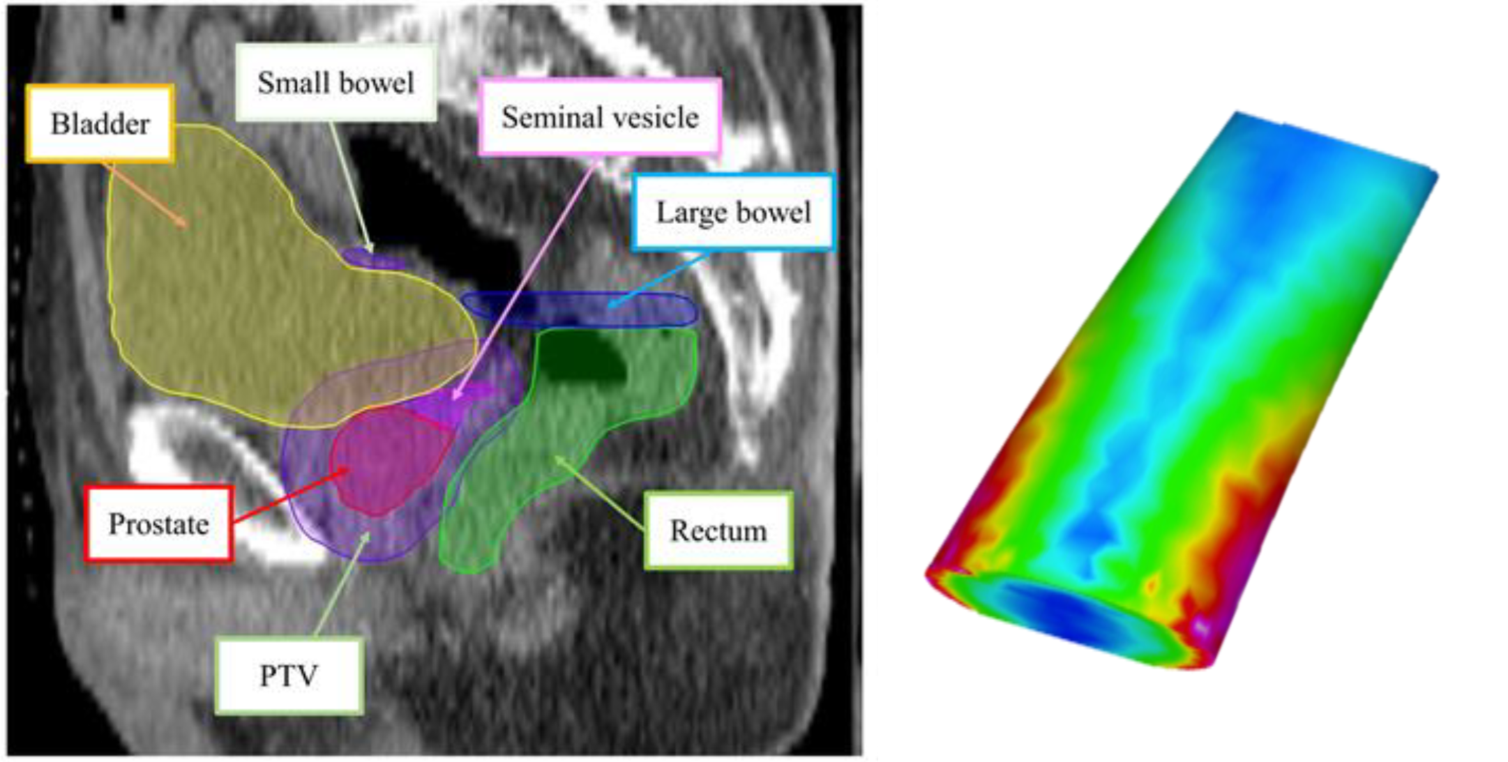
Figure 12:Use case for triangulation: computing the surface dose of triangulated representation of anatomical structures (e.g. rectum wall) in radiotherapy, image courtesy of Prof. Gabor Fichtinger at Queen’s University, Canada.
The area of a triangle is half of the area of a parallelogram with the same base length and height.
:label: fig_area_triangle :alt: Area of a triangle :align: center :width: 80%
The area of a triangle as half of area of a parallelogram that has the same base length and height, image courtesy of Wikimedia Commons here, accessed January 9, 2026.
If a triangle is presented by three points $b$, $c$, with the angle $\alpha$ between them, The base of the triangle can be taken as $c$ and the height of the triangle, $h$, is equal to the length of $b$ multiplied by $\sin{\alpha}$:

```{figure} ./../images/002/fig_triangle_vectors.png
:label: fig_area_triangle_vectors
:alt: Area of a triangle
:align: center
:width: 80%

A triangle represented by 2 vectors $b$ and $c$, separated by an angle $\alpha$. The **base** is $c$ and the **height** is $h$.
That is, the area of the triangle is calculated as: $$
$$
But is the length of the cross product ! Thus, the area of a triangle can be computed as:
A = np.array([ 3, 0, 0 ])     # this is a row vector
B = np.array([ 0, 4, 0 ])
A = A.reshape(-1,1)           # this is now a column vector
B = B.reshape(-1,1)

Area = 0.5 * np.linalg.norm( np.cross(A, B, axis=0) )

print( "Area of the triangle is:", Area)
Area of the triangle is: 6.0
For visualization and other implementations, consult the following tutorial.
Dot product of Two Vectors
Dot product, or the inner product, of two vectors, is the sum of the element-wise product. The final value is a scalar and not a vector:
where is the angle between these two vectors.

Figure 13:Illustration showing how to find the angle between vectors using the dot product, image courtesy of Wikimedia Commons here, accessed January 9, 2026.
Note the properties of dot product:
Commutative,
Not Associative (but why?): , but
Distributive with addition:
It can be trivially shown that the length of a vector is just the square root of the dot product with itself:
Because the dot product is related to the cosine of the angle between two vectors, we can use it to evaluate if two vectors are orthogonal with eather other: if their dot product is 0, implying that is 0, these two vectors must be perpendicular:
A = np.array([ 3, 0, 0 ])     # this is a row vector
B = np.array([ 0, 4, 0 ])
A = A.reshape(-1,1)           # this is now a column vector
B = B.reshape(-1,1)

# np.dot(A,B) ## won't work as numpy assume row vector. Instead, use this:
print("The dot product is:", A.T@B)
The dot product is: [[0]]
Angle between Two Vectors
Given two vectors and with the angle in between, we now have 2 ways to calculate the angles:
Via dot product
or via cross product
Given a situation, which one should you use? One recommendation is to consider the slope of the and function and avoid the flat area of the curve:

Figure 14:Sine and cosine as function of the angle, image courtesy of Wikimedia Commons here, accessed January 9, 2026.
Around use sine, i.e. cross product,
Around use cosine, i.e. dot product
A more robust method is to use both the cross and dot products:
atan2( norm( cross(u,v)), dot(u,v))Here is an example:
a = 1e-10                               # a small number
u = 4.0 * np.array([[1],                # a non-unit vector along the x-axis
                    [0],
                    [0]])
v = 5.0 * np.array([[ math.cos(a) ],    # a non-unit vector different from u
                    [ math.sin(a) ],    # by a very small angle
                      [0]])

dotproduct = ((u.T@v)[0])[0]
crossproduct = np.linalg.cross( u, v, axis=0 )
print( "The angle in radian between 2 vectors is:\n", a )
print( "The angle computed using dot product (cosine):\n",
      math.acos( dotproduct / ((np.linalg.norm(u))*(np.linalg.norm(v)))) )
print( "The angle computed using cross product (sine):\n",
      math.asin( np.linalg.norm(crossproduct) / ((np.linalg.norm(u))*(np.linalg.norm(v)))) )
print( "The angle computed using both cross and dot products: \n",
      math.atan2( np.linalg.norm( crossproduct ), dotproduct ))
The angle in radian between 2 vectors is:
1e-10
The angle computed using dot product (cosine):
0.0
The angle computed using cross product (sine):
1e-10
The angle computed using both cross and dot products:
1e-10
An use case is to determine the Cobb angle, a measurement of the bending disorders of the vertebral column, for patients with scoliosis based on an x-ray image:
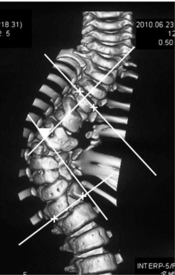
Figure 15:Cobb angle is determined from an frontal view of surface-rendered CT volume based on the angle between two vectors, image courtesy of Prof. Gabor Fichtinger of Queen’s University, Canada.
Vector Representation of a Line
There are many ways to represent a line. In fact, the appropriate representation often depends on mathematical convenience and the definition of a line. In CAS, a line could mean
an oriented line: a line with a point on the line (i.e. the origin) and a direction (often represented by a unit vector)
a line segment: a line with length
can be represented by the two end points of the line segment, or
can be represented by one of the end point plus a vector of the known length
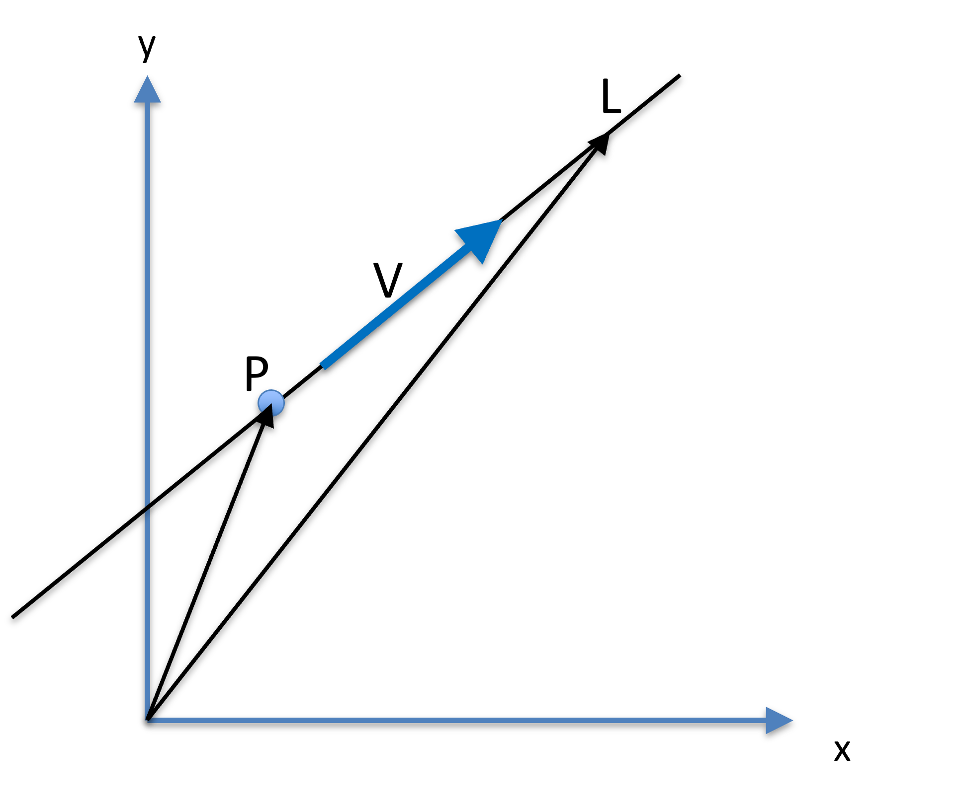
Figure 16:A line can be presented by a fixed point , a unit dictional vector , and a parameter , where another point on the lie is .
Parameterized Line
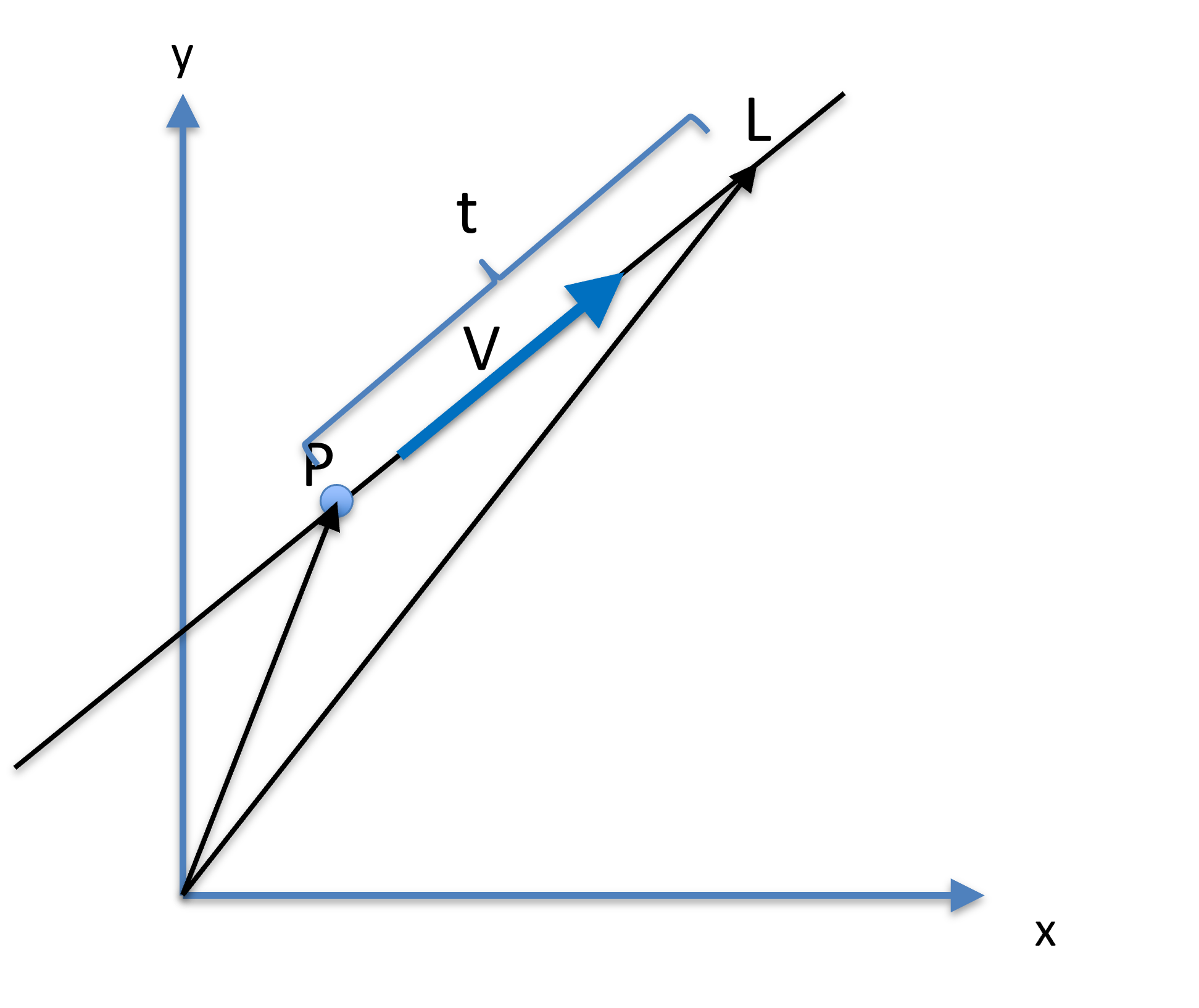
Figure 17:A line can be presented by a fixed point , a unit dictional vector , and a parameter , where another point on the lie is .
Let be a point on a line, and a unit vector be the direction (orientation) of the line. Another point on the line can be parameterized as:
where is a scalar, effectively specifying how far is from . Specifically, is calculated as
The orientation vector does not need to be a unit vector, but mathematically convenient if it is. The range of specify the type of the line:
Infinite line:
Ray:
Line Segment:
To understand what the parameterizing parameter is, let’s rearrange the equation of the line:
Because , i.e. was normalized, then
That is, if is a unit vector, the parameter measures the distance between the fixed point and the running point .
P = np.array([[0],          # a fixed point on the line
              [0],
              [0]])
v = np.array([[1],          # orientation of the line as a unit vector
              [0],
              [0]])
t = 3.0                     # line parameterization
L = P + t * v               # another point on the line
print( L )
[[3.]
[0.]
[0.]]
Line Defined by Two Points
Give two points and on a line, the orientation of the line can be determined by
The orientation unit vector is
That is, the orientaiton of the line is determined by substracting one point from another; the order of which is important as it determines the direction of the line. The orientation vector is normalized for mathematical convenience.
P = np.array([[0],          # a fixed point on the line
              [0],
              [0]])
L = np.array([[3],          # another point on the same line
              [0],
              [0]])
dir = L-P                   # orientation of the line
v = dir/np.linalg.norm(dir) # normalized orientation, i.e. a unit vector
print(v)
[[1.]
[0.]
[0.]]
Distance of a Point from a Line
The distance between a point and a line is defined as the shortest distance beween to any points on . Suppose a line is represented by the fixed point on the line and a unit orientation vector . The length is the distance between point and and is the length of the hypotenuse of a right-angle triangle. The projection of onto is the adjacent of the right-angle triangle, with the angle denoted as . The distance between the point and line is the length of the opposite of the right-angle triangle.
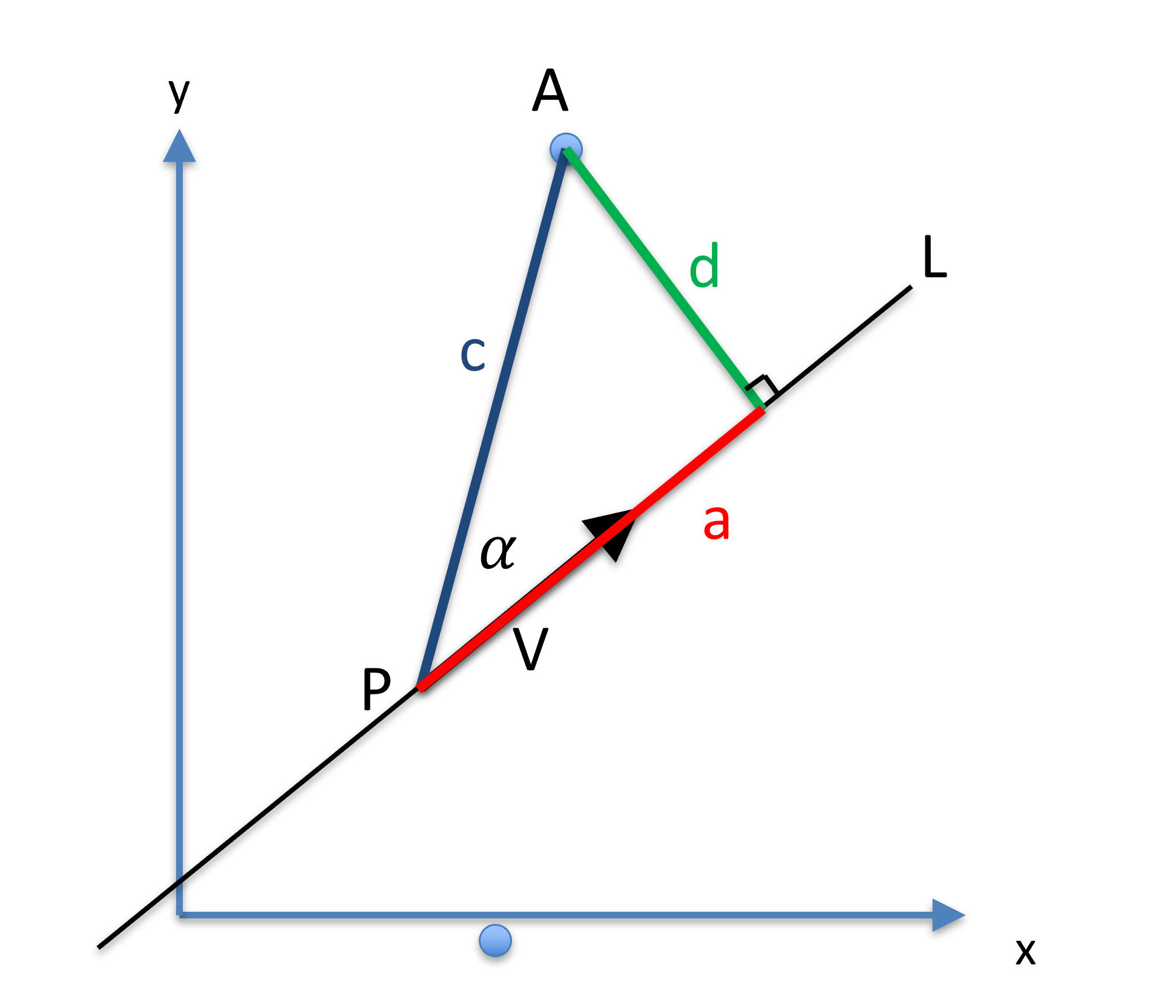
Figure 18:The distance between a point and line can be calculated based a triangle being formed.
Using this right-angle triangle, one can calculate the distance using:
P = np.array([[0],              # a fixed point on the line
              [0],
              [0]])
v = np.array([[1],              # a unit vector representing the orientation of the line
              [0],
              [0]])
A = np.array([[3],              # a point NOT on the line
              [4],
              [0]])

c = np.linalg.norm( A-P )
a = np.linalg.norm( v.T@(A-P) )
d = math.sqrt( (c+a)*(c-a) )    # just a more efficient way of calculating c*c-a*a
print(d)
4.0
This formulation calculates the distance between a point and an line without knowing which point on the is the closest to . However, since we know , the length of the adjacent of the right-angle triangle, we can determine which point on is closest to A:
Q = P + a*v                     # Q is a point on line L that is closest to point A
print( Q )
print( np.linalg.norm(A-Q))     # The length of the vector AQ
[[3.]
[0.]
[0.]]
4.0
A use case in CAS: suppose we want to insert a biopsy needle (a line) into the center of the prostate (a point) to take a sample; one may wish to know how far away the biopsy needle is to the intented target.

Figure 19:Screen capture in ultrasound-guided prostate biopsy navigation. Computing the needle placement error as the distance between the planned target (a point) and the actual needle path observed in ultrasound (a line), image courtesy of Prof. Gabor Fichtinger at Queen’s University, Canada.
Plane
A plane is represented by a point on the plane and the surface normal of the plane. For mathematical convenience, the normal of the plane is normalized with a length of 1.
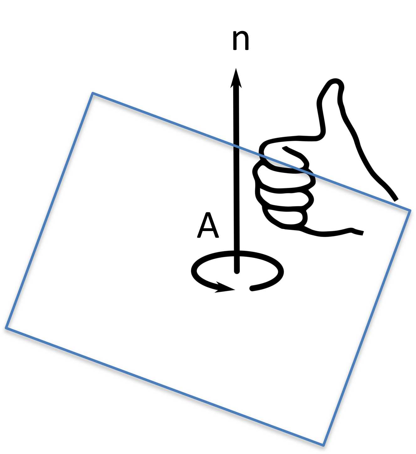
Figure 20:The distance between a point and line can be calculated based a triangle being formed.
Given 3 points , , and on a plane, the plane normal vector can be computed by their cross product:
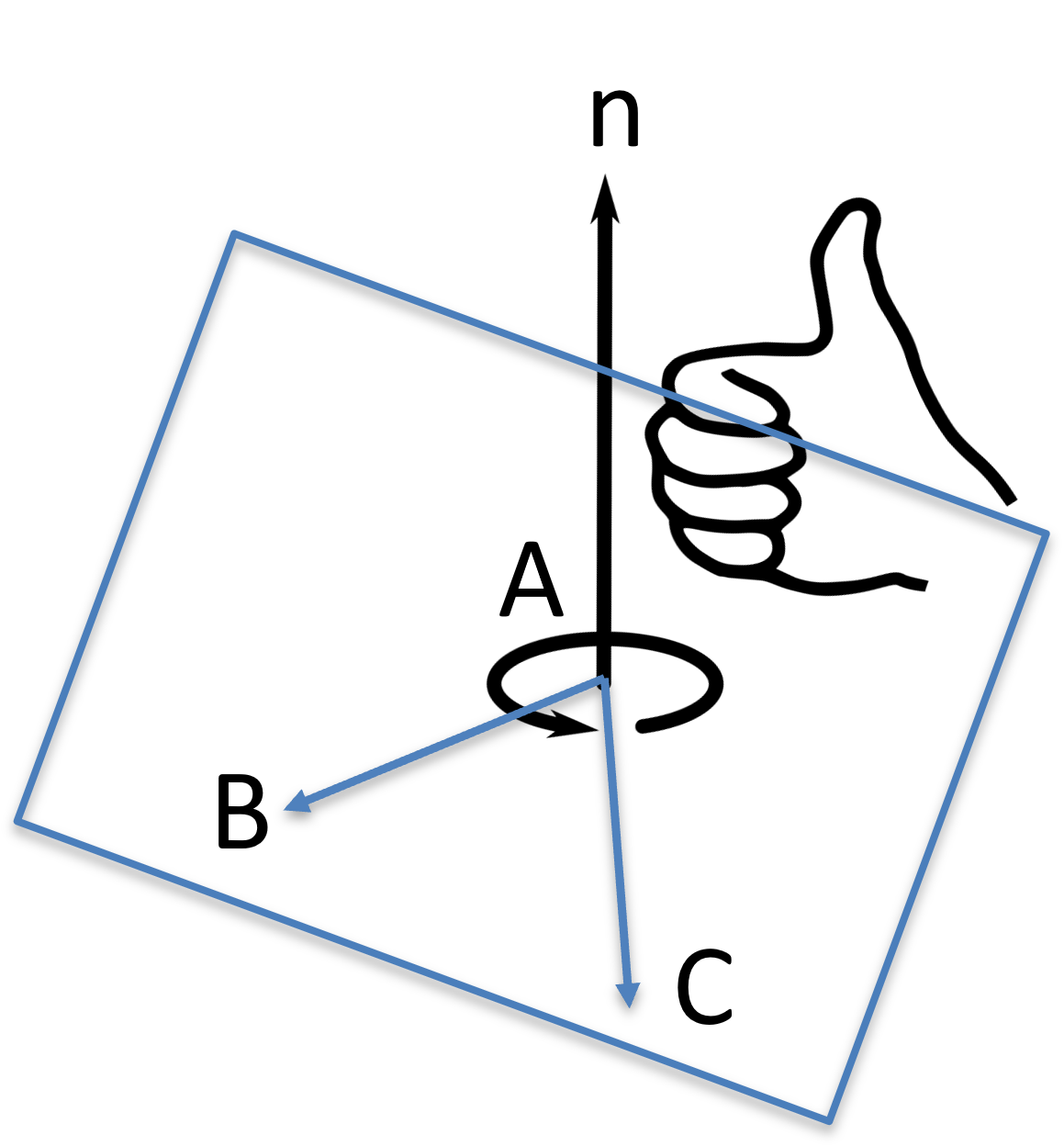
Figure 21:The distance between a point and line can be calculated based a triangle being formed.
A = np.array([[0],              # a point on the plane
              [0],
              [0]])
B = np.array([[1],              # a point on the plane
              [0],
              [0]])
C = np.array([[0],              # a point on the plane
              [1],
              [0]])

dir = np.linalg.cross( (B-A), (C-A), axis=0 )
n = dir/np.linalg.norm(dir)
print( "plane normal vector is:\n", n)
plane normal vector is:
[[0.]
[0.]
[1.]]
Distance from a Plane
The distance between a point from a plane , where is a unit vector specifying the normal of the plane, and is a point on the plane, is the length of the projection of to the surface normal :
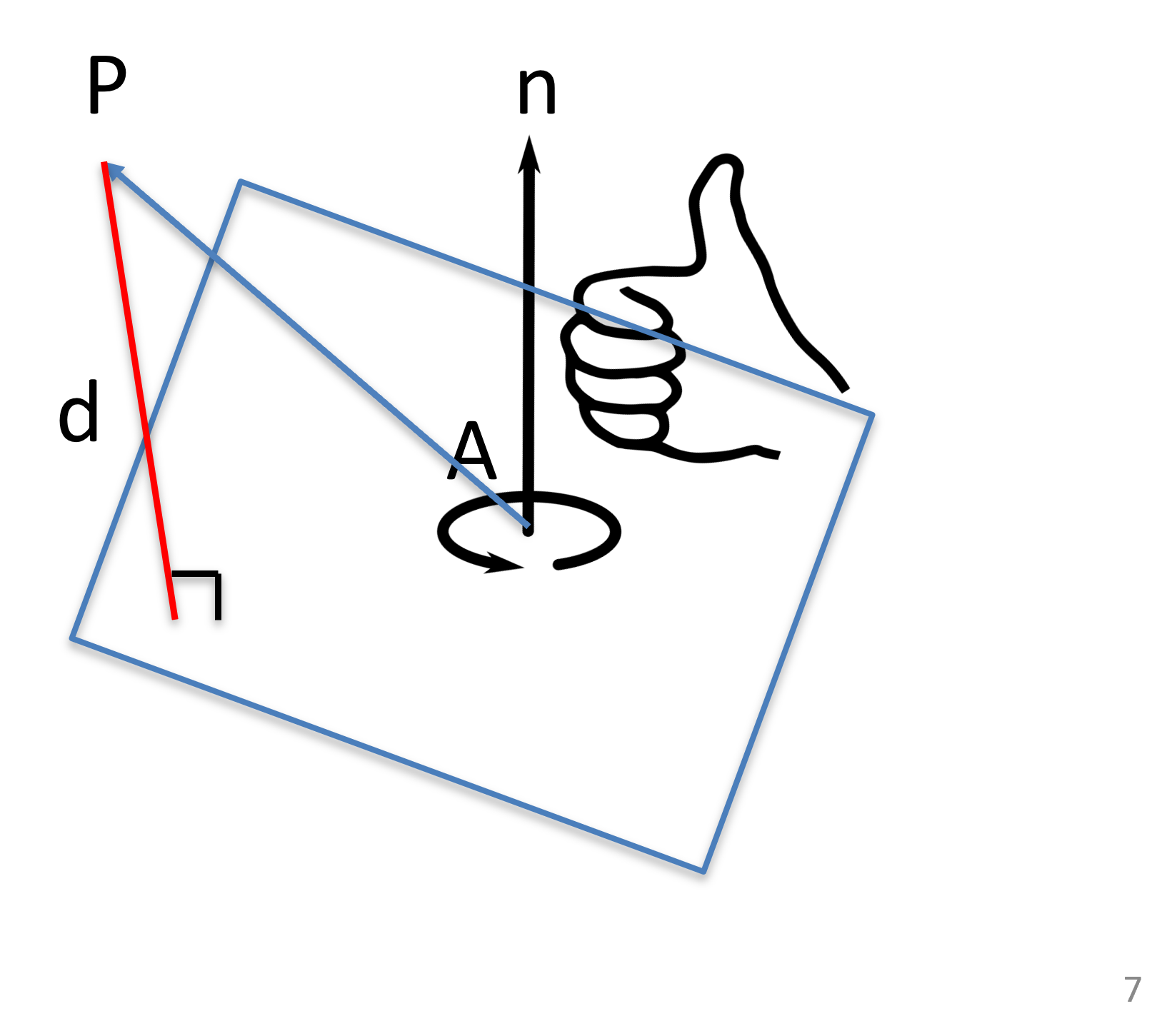
Figure 22:The distance between a point and plane can be calculated as a dot product.
Notice the plane normal has a direction:
if , then is above the plane,
if , then is below the plane,
if , then is on the plane.
A = np.array([[0],                 # a point on the plane
              [0],
              [0]])
n = np.array([[0],                 # plane normal
              [0],
              [1]])
P = np.array([[3],                 # a point
              [4],
              [5]])

d = (n.T@(P-A))[0][0]
print("The distance is:", d)
The distance is: 5
Intersection of Line and Plane
The intersection between a line, , and a plane, can be calculated as the following.
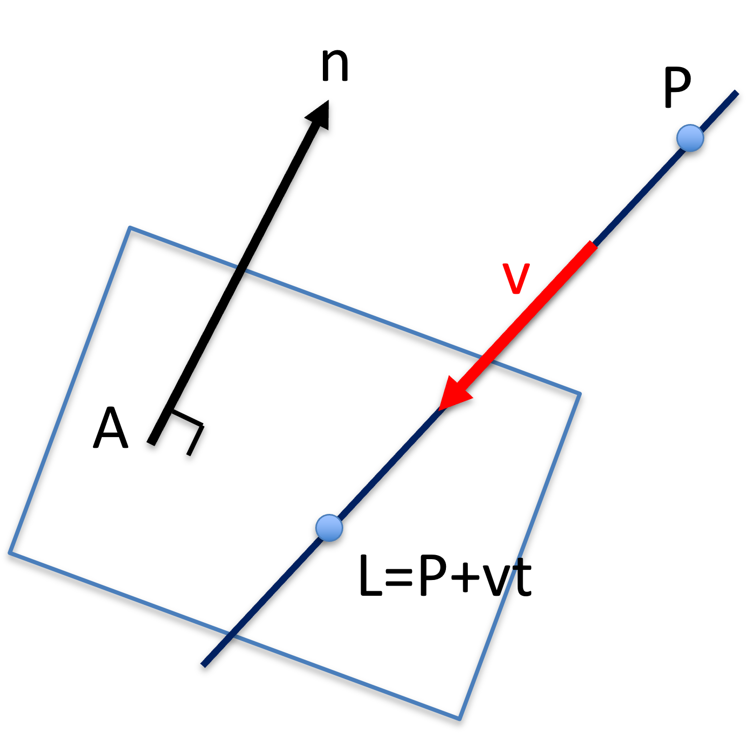
Figure 23:The intersection between a parameterized line to a plane .
Assuming the line is parameterized with :
When intersects with the plane, i.e. is on the plane, then
Substitute Eqn.(23) into Eqn.(24):
Using the distributive property of dot product, one obtains:
Rearrange for :
Substitute back to Eqn.(23) to obtain the intersection point .
For visualization and other implementations, consult the following tutorial.
One of the use case involves the use of X-ray or Fluoroscopy where X-ray, originated from a point source, is treated as a line, and the image detector is the plane.
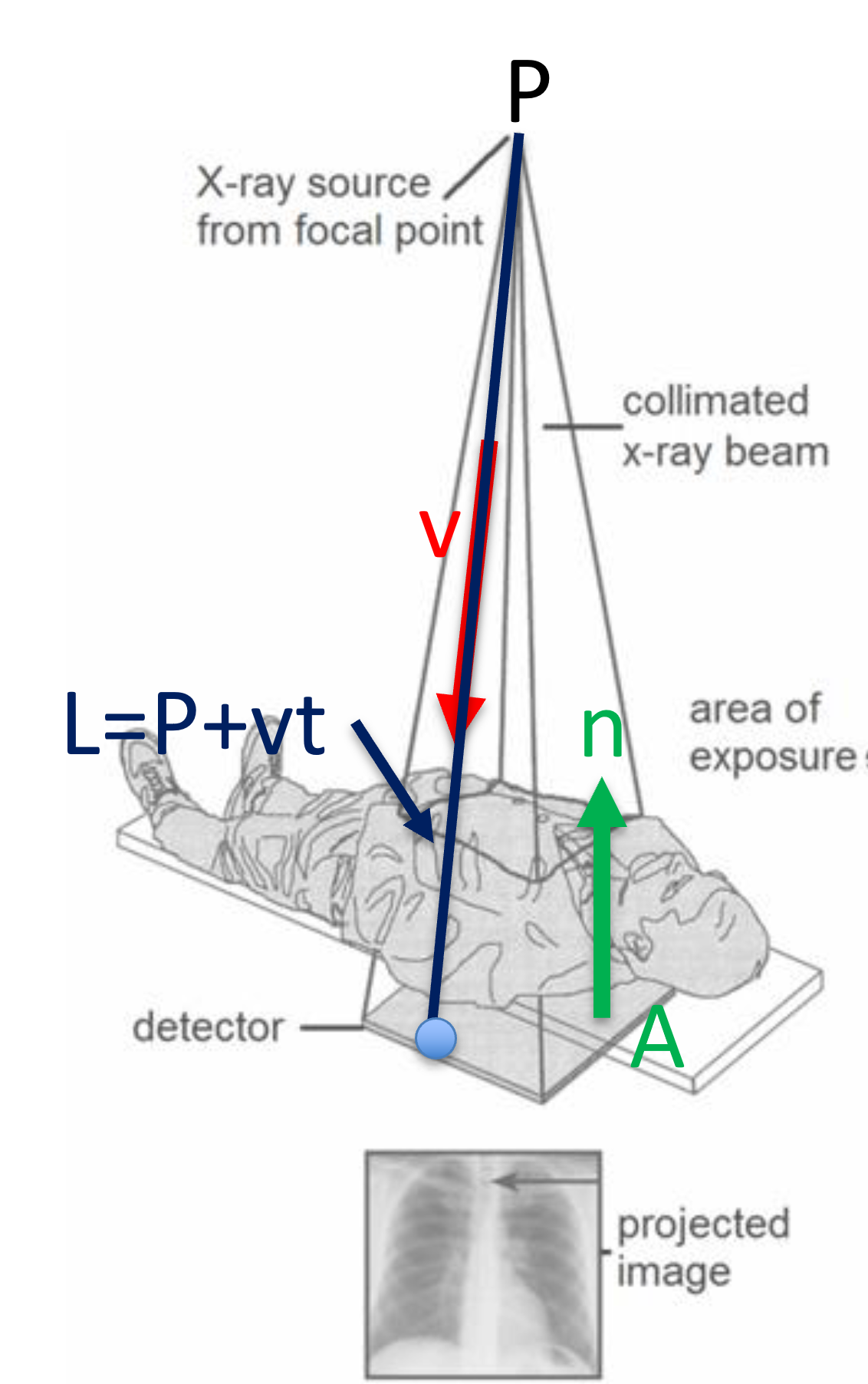
Figure 24:The intersection between an X-ray to the detector as a use case for calculating the intersection between a line and a plane, image courtesy of Prof. Gabor Fichtinger at Queen’s University, Canada.
Intersection of Lines in 3D
Intersection of lines in 3D is common in motion analysis, often involved the usa of stereo camera of bi-plane fluoroscopy. In Figure 25, the X-ray source is treated as a Pinhole camera, and the principle of triangulation is used to localize an object.
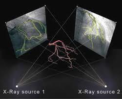
Figure 25:Biplane X-ray target reconstruction, image courtesy of Prof. Gabor Fichtinger at Queen’s University, Canada.
Let two lines be represented parametrically:
Expanding for each components, one obtains:
and
where
If lines intersect with each other, they share a common point in space. That is,
for some and , and
There and are unknown. You should note that these are 3 equations with 2 unknowns, thus, in general, two lines do not intersect in 3D.
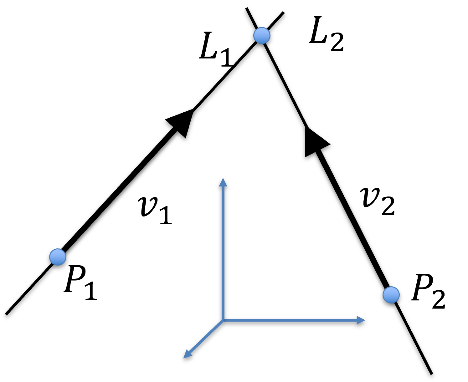
Figure 26:Intersection of 2 lines in 3D.
In other words, 2 lines intersect with each other if one of these three equations cancels out. That is, if one of the equations can be expressed as a linear combination of the other two: they lie on a common plane. However, this does not happen in general, either because two lines in fact do not intersect with each other, or they do but numerically the equations above cannot be satisfied due to digital representation.
But we can in fact calculate a “symbolic intersection”: find the shortest distance between two lines and the midway point.
The symbolic intersection point is a point that is equal distance from both lines. It can be computed in 3 steps:
Find a line that is perpendicular to both lines,
Find the intersection of line with both lines and , and
Find the middle point on
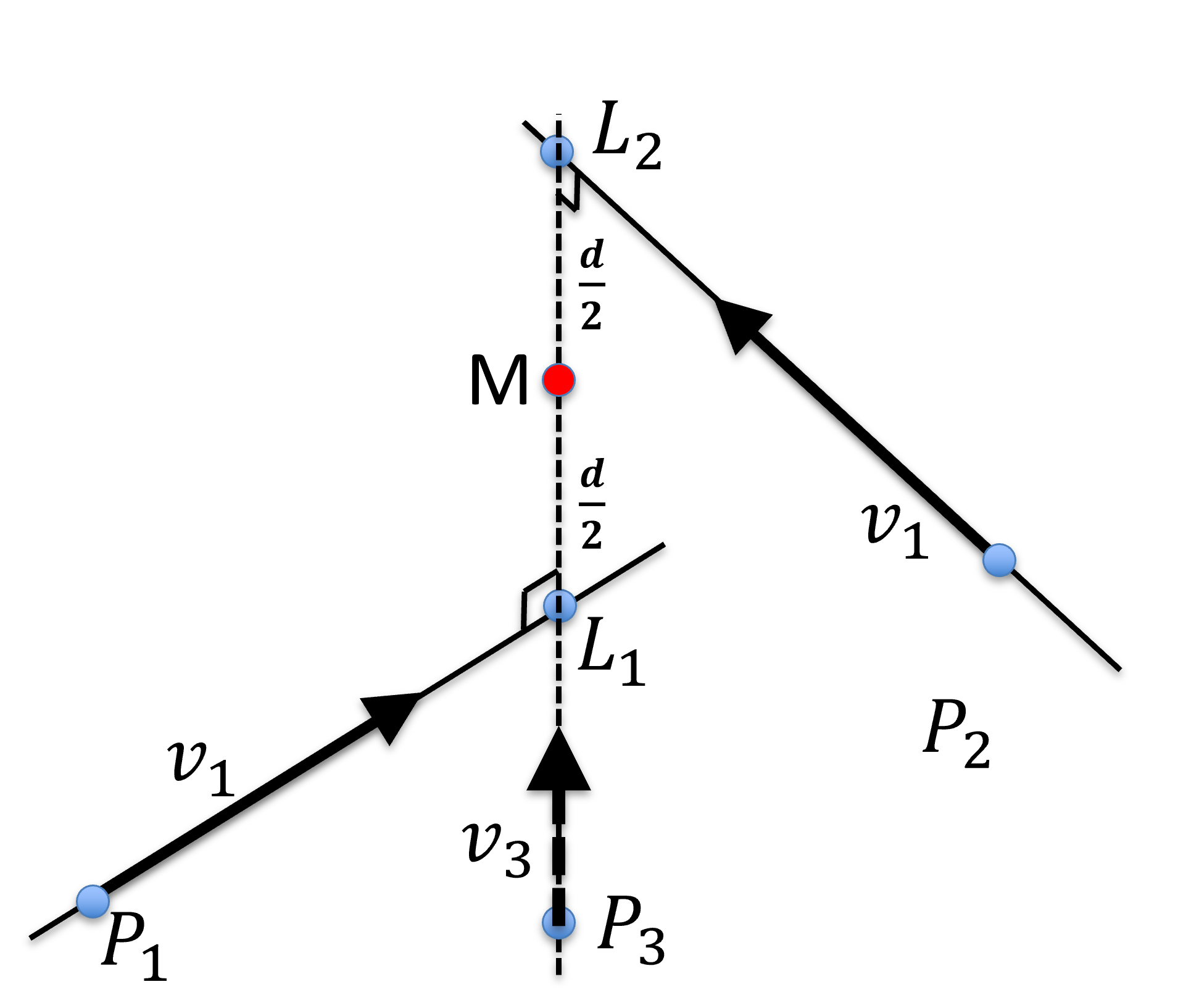
Figure 27:Symbolic intersection, , of 2 lines in 3D. is perpendicular to both and and is mid-way from and with a distance .
The distance between the mid-way point is denoted as the Residual Eerror Metric (REM), which is , and is the distance between lines and .
Line 3 is perpendicular to the other two lines, thus, its directional vector can be computed as the cross product of the other two directional vectors:
The length of is normalized to be 1, again, for mathematical convenience.
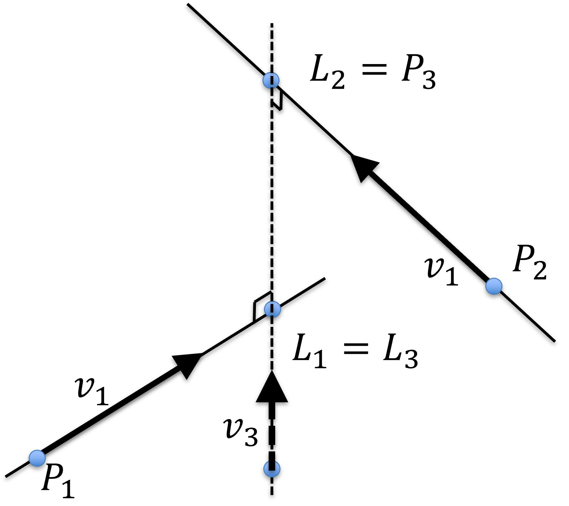
Figure 28:Symbolic intersection, , of 2 lines in 3D. is perpendicular to both and and is mid-way from and with a distance .
As such, the fixed point and the parameterized point on this line can be designate as
Because the equations for all three lines are:
Substituting Eqn.(35) and Eqn.(36) into Eqn.(39) yields:
After rearrangement:
and expanding it to each of the 3 dimensions:
where , and are unknown. Now there are 3 equations and 3 unknown, implying that a unique solution does exist.
These equations can be represented using matrices:
The unknown , and can be solved using
Algebraic substitution, or
Matrix inversion (shown below)
Once , , and are calculated, substitute them back to
to solve for and . Note that
and
The REM, which is the distance of from either or is:
P1 = np.array([[0],                 # a point on z=0 plane
              [0],
              [0]])
v1 = np.array([[1],                 # line orientation +x
              [0],
              [0]])
P2 = np.array([[0],                 # a point on z=5 plane
              [0],
              [5]])
v2 = np.array([[0],                 # line orientation +y
              [1],
              [0]])

v3 = np.linalg.cross( v1, v2, axis=0 )


V = np.zeros((3,3))                 # construct the 3x3 matrix
V[:,0] = -1*v1.reshape(1,3)
V[:,1] =    v2.reshape(1,3)
V[:,2] =    v3.reshape(1,3)

P = P1-P2
t = np.matmul( np.linalg.inv(V), P)

# solve for L1 and L2
L1 = P1 + t[0] * v1
L2 = P2 + t[1] * v2
M = 0.5 * (L1+L2)
REM = .5 * t[2][0]
print("The symbolic intersection is: \n", M,
      "\nwith REM of ", REM)
The symbolic intersection is:
[[0. ]
[0. ]
[2.5]]
with REM of -2.5
Symbolic Intersection of Lines in 3D
One utility of computing the intersection of lines in 3D is to find the centre of the volume in a reconstructed CT volume.
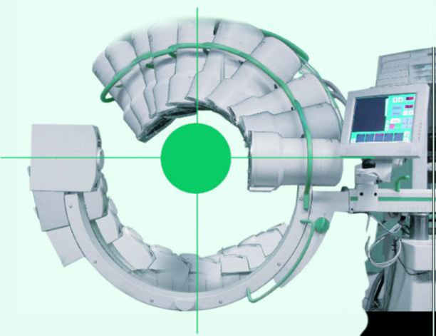
Figure 29:Rotational X-ray Reconstruction, where center of the imaged volume is the intersection of multiple lines in 3D.
First, write the equation for all ines
The the problem of computing the symbolic intersection can be posed as a least-square optimization with the cost function of:
and compute where is the minimum.
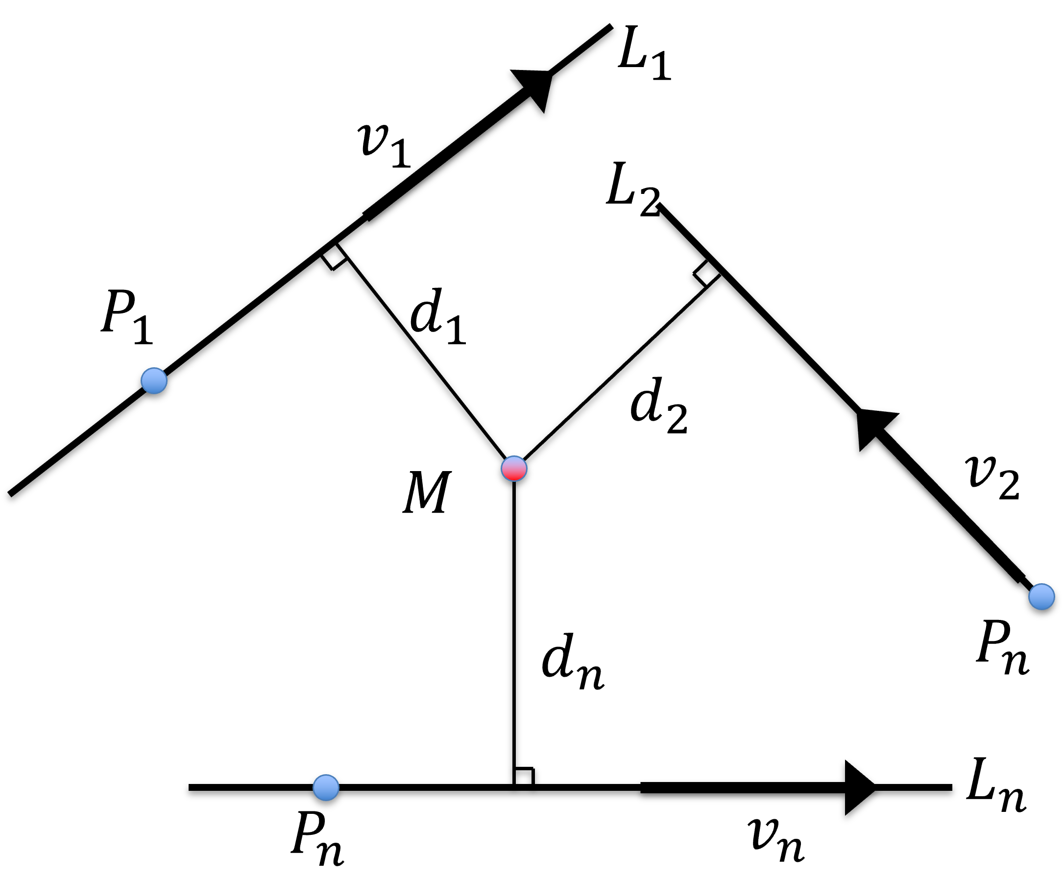
Figure 30:Intersection of lines in 3D where the point is the symbolic intersection, having the shortest sum of distance from all lines.
Throughout the optimization process, one should always be mindful of deriving and monitoring error metrics including Root Mean Square (RMS), average (Avg), and standard deviation (STD), and use them a means to detect and remove Outlier. For example, an outlier can be defined as:
or
(typically or ). Once outlier is detected, they are moved from the population and the optimization is recomputed, so are the error metrics. This process is repeated until no outlier is left, or the input data is completely removed (a bad situation).
One easy way to approximate the symbolic intersection point is to compute pairwise intersections for all pairs and approximate as the average, i.e. COG, of these pairwise intersections:
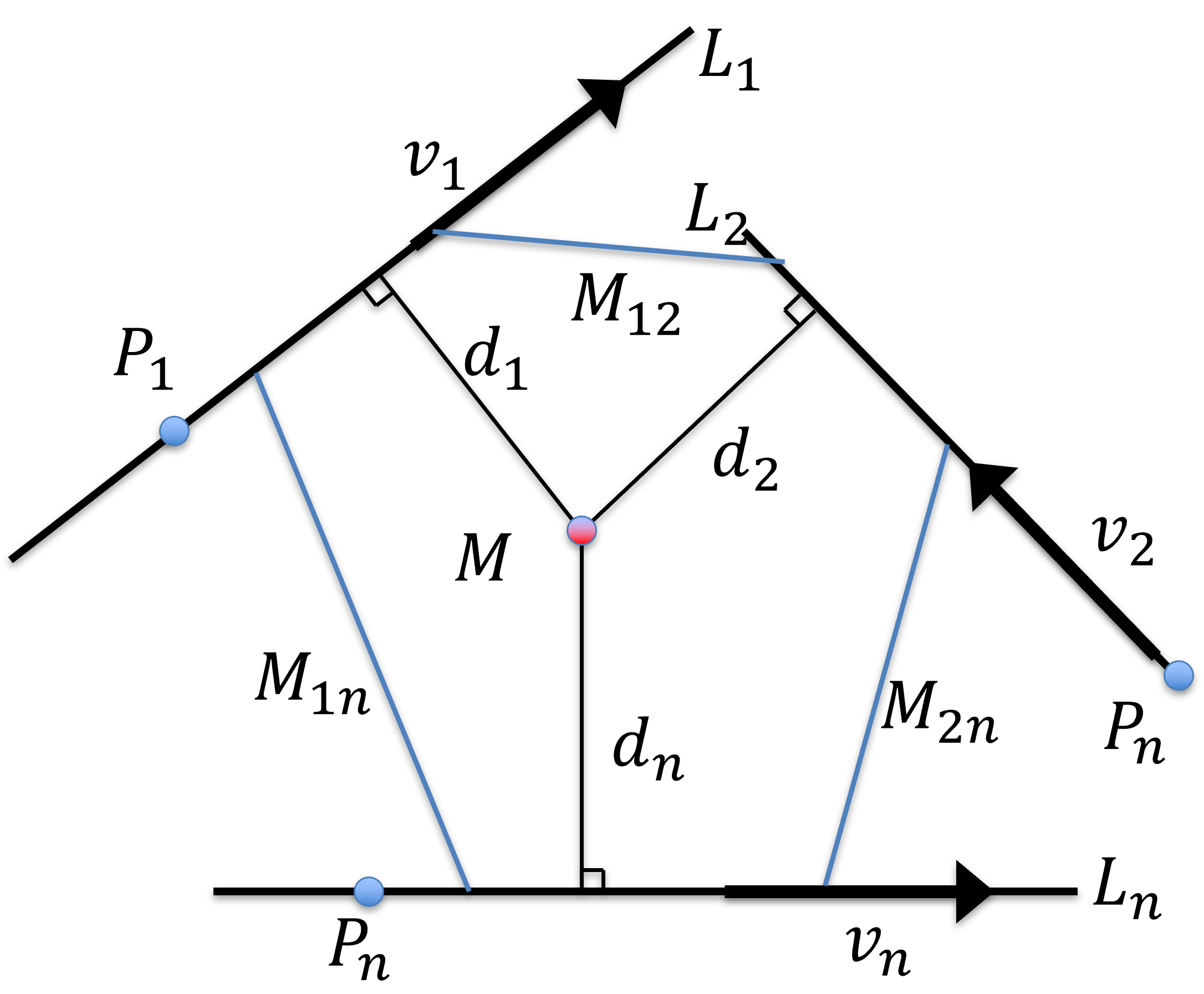
Figure 31:Approximation of the symbolic intersection of lines in 3D as the centroid of the pair-wise line intersections.
If the input is decent, i.e. no outliers and all lines come very close, this simple average is almost as good as the proper least square minimum.
In fact, there is indeed no outlier, a closed-form solutoin exist. Let be the fixed point on line and be the unit vector along the line, then can be calculated as:
P1 = np.array([[5],                 #
              [0],
              [0]])
v1 = np.array([[1],                 #
              [0],
              [0]])
P2 = np.array([[0],                 #
              [0],
              [9]])
v2 = np.array([[0],                 #
              [1],
              [0]])
P3 = np.array([[1],                 #
              [1],
              [0]])
v3 = np.array([[0],                 #
              [0],
              [1]])

# initialization
I = np.identity(3)
Sum1 = np.zeros((3,3))
Sum2 = np.zeros((3,1))
# 1st point
Sum1 += I-v1@v1.T
Sum2 += np.matmul(I-(v1@v1.T), P1)

# second point
Sum1 += I-v2@v2.T
Sum2 += np.matmul(I-(v2@v2.T), P2)

# third point
Sum1 += I-v3@v3.T
Sum2 += np.matmul(I-(v3@v3.T), P3)

# solution
M = np.matmul(np.linalg.inv(Sum1), Sum2)
print(M)
[[0.5]
[0.5]
[4.5]]
This is a good time to learn about iterative solution vs a closed-form solution. In mathematics, a closed-form solution is often optimal with regarding to certain error metric, in this case, the Euclidean distance. However, closed-form solution are sensitive to outlier.
On the other hand, iterative solution (i.e. via optimization) may not reach a solution that is optimal with respect to the given error metric. However, it allows rooms to integrate outlier detection and removal naturally during the iterative process.
Cartesian Equations of Sphere and Ellipsoid
Spheres and ellipsoid are often used to approximate the size of anatomical structures, such as a tumour, in 3D from medical imaging.
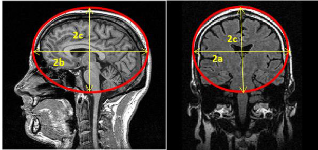
Figure 32:Sphere and ellipsoid are used to determine the size of anatomical structures in 3D, image courtesy of Prof. Gabor Fichtinger at Queen’s University, Canada.
A sphere is represented by its center and the radius , with the corresponding equation of:
which can be used to test if a point is on the surface of the sphere or not.
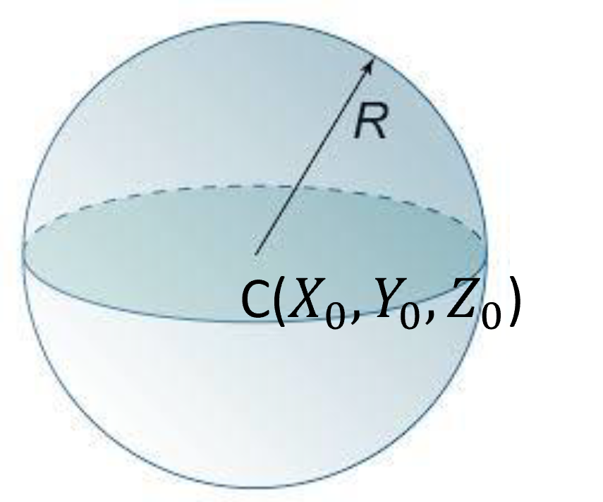
Figure 33:A sphere is defined by its center and a radius .
An ellipsoidis represented by its center and the lengths of principal axes :
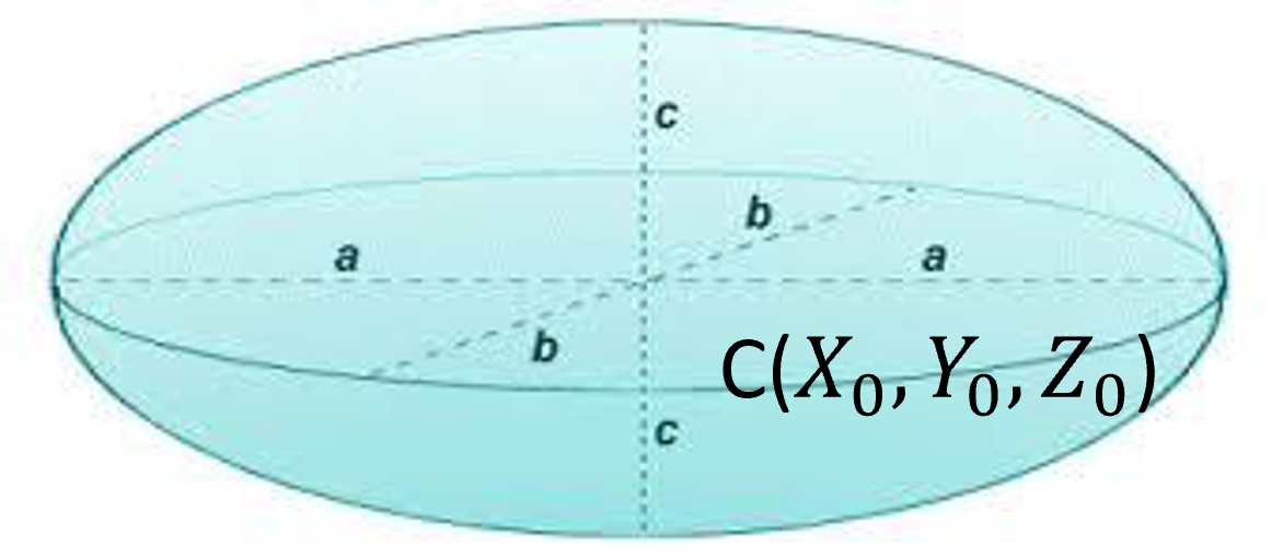
Figure 34:An ellipsoid is defined by its center and the lengths of principal axes.
mathematically represented as
Intersection of Line and Sphere/Ellipsoid
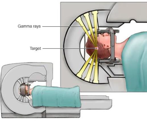
Figure 35:An ellipsoid is defined by its center and the lengths of principal axes.
Let the line be presented by the being the fixed point on the line, a unit vector representing the direction of the line, and being the scalar.
And the equation of the sphere is:
where is a point on the surface of the sphere, is the center of the sphere and is the radius. If the point on the line intersects with the sphere, must also satisfy the equation of the sphere:
which can be evaluated using dot product:
Using the distributive property of dot product and rearrange the terms:
which has the form of a quadratic formula:
where $$
$$
and can be solved as:
Because is a unit vector, the above solution can be simplified as:
Eqn.(63) is worth investigating: let be the term inside the square root:
If , there is no solution: the line does not intersect the sphere,
If , there is exactly one solution: the line is tangent to the sphere,
If , there are 2 solutions: the line intersect the sphere in 2 locations (i.e. going through)
C = np.array([[0],                  # centre of a sphere
              [0],
              [0]])
R = 5                               # radius of the sphere
v = np.array([[-1],                  # orientation of a line (unit vector)
              [0],
              [0]])
P = np.array([[10],                  # a fixed point on the line
              [0],
              [0]])

PC=P-C
print(PC)
determinant = ((v.T@PC)*(v.T@PC) - PC.T@PC + R*R)[0][0]
print(determinant)
a = (-1 * v.T@PC)[0][0]

if determinant < 0:
    print("no solution")
elif determinant == 0:
    t = a
    L = P + t * v
    print("one intersection at: \n", L)
else:
    t = a + math.sqrt(determinant)
    L = P + t * v
    print("one intersection at: \n", L)
    t = a - math.sqrt(determinant)
    L = P + t * v
    print("one intersection at: \n", L)
[[10]
[ 0]
[ 0]]
25
one intersection at:
[[-5.]
[ 0.]
[ 0.]]
one intersection at:
[[5.]
[0.]
[0.]]
For visualization and other implementations, consult the following tutorial.
Ellipsoid
Similiarly, the intersection between a line and an ellipsoid can be expressed as an equation with a quadratic form. For completeness, let the line be presented as:
where is a fixed point on the line, be the unit orientation vector, a scalar, and is the parameterized point on the same line.
An ellipsoid is defined by its center and the lengths of principal axes, mathematically represented as
The point on the line is on the surface of the ellipsoid when
Expand and simplifying:
which is a quadratic equation of . Similar to the case of intersection between a line and a sphere, there will be three cases:
The line does not intersect with the ellipsoid,
The line intersects with the ellipsoid at one location, i.e. the line is tangent to the ellipsoid, or
The line intersects with the ellipsoid at two locations.
Below, you should try to implement this equation and come up with a evaluation case to verify your implementation.
For visualization and other implementations, consult the following tutorial.
Fitting Points to Sphere in 3D
One if the critical use case in CAS for fitting points to a sphere in 3D is tool-tip calibration where, when a tracking sensor is attached to a (as an example) to a surgical drill, the location of the drill tip can be determined with respect to the tracking sensor via pivot calibration.
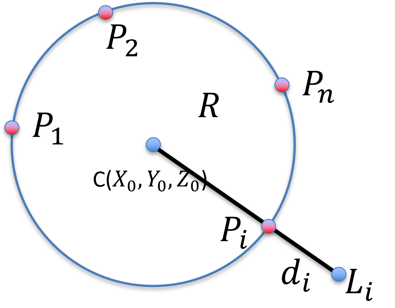
Figure 36:Fitting a set of measured points to a sphere, in 3D. is the set of points, one hope to recover the center and the radius of the sphere.
In pivot calibration, where the tip of the surgical drill remains stationary but the body of the surgical drill pivot about this stationary point, the path of any point on the body of the surgical drill lies on the surface of a sphere (with an error margin ). Thus, the problem of fitting a set of measured points to a sphere centered at with a radius can be treated as a least square optimization, with the error to minimize being the sum of square distance of all measured points from the surface of the sphere:
and it to find an optimal . Akin with other optimization approach, you should always compute an error metric, for examples RMS, Avg, and STD, and set rules for outliers to maintain data integrity.
Many closed for solutions also exist and are suitable if there is no data outliers. Al-Sharadqah & Chernov (2009) provides a good background materials from a pure mathematical point of view (but for fitting circle in 2D). A mathod utilizing the Singular Value Decomposition (SVD) with hyperaccuracy and no essential bias is coded in Matlab below.
function Par = HyperSVD( XYZ )
%
% Algebraic sphere fit with "hyperaccuracy"
% i.e. with zero essential bias
%
%
% INPUTS:  XYZ - 3xn matrix of 3D points that are (noisy) measurements of
%                points laying on a sphere
%
% OUTPUT:  Par = [ a b c R ] is the fitting sphere,
%              centered at ( a, b, c ) with radius R
%
% Based on the paper by
%
%     Error analysis for circle fitting algorithms
%     A. Al-Sharadqah and N. Chernov
%     Electronic Journal of Statistics
%     Vol. 3, 2009
%     page 886--911
%
% Elvis C.S. Chen
% chene@robarts.ca
%
% Jan. 30, 2013
%
% heavily based on the original 2D circle fit by Chernov
%

% assume row vectors
centroid = mean( XYZ, 2 );

% de-mean and calculate the squares
X = XYZ(1,:) - centroid(1);
Y = XYZ(2,:) - centroid(2);
Z = XYZ(3,:) - centroid(3);
ZZ = X.*X + Y.*Y + Z.*Z;

% construct the matrix Z based on equation (21)
ZZZ = [ ZZ' X' Y' Z' ones( length(Z),1) ];
[U,S,V] = svd( ZZZ, 0 );

if ( S(5,5)/S(1,1) < 1e-12 ) % singular case
    A = V(:,5);
else
   % consult page 904 for an algorithm describing the following code
   R = mean( ZZZ );

   % construct the constrain matrix N based on equation (87)
   %
   % this is stupid, R(2:4) are zero since it is de-mean already
   %N = [ 8*R(1) 4*R(2) 4*R(3) 4*R(4) 2; ...
   %      4*R(2) 1      0      0      0; ...
   %      4*R(3) 0      1      0      0; ...
   %      4*R(4) 0      0      1      0; ...
   %      2      0      0      0      0 ];
   %N = eye(5);
   %N(1,1) = 8*R(1);
   %N(1,5) = 2;
   %N(5,1) = 2;
   %N(5,5) = 0;

   % we can build the inverse of N directly
   invN = eye(5);
   invN(1,1) = 0;
   invN(1,5) = 0.5;
   invN(5,1) = 0.5;
   invN(5,5) = -2*R(1);
   W = V * S * V';
   %[E,D] = eig( W * inv(N) * W );
   [E,D] = eig( W * invN * W );
   [Dsort,ID] = sort(diag(D));
   Astar=E(:,ID(2)); % find the smallest positive eigen value
   A = W\Astar;
end

% recover the natural parameter based on equation (12)
Par = -.5 * A(2:4)'/A(1) + centroid'; % center
Par = [ Par, sqrt( A(2)^2 + A(3)^2 + A(4)^2 - 4*A(1)*A(5))/abs(A(1))/2 ];
end
Fitting Points to line in 3D
Fitting a set of measured points in 3D to a line effectively finds the orientation of the line. Using the tracked surgical drills as an example,
The pivot calibration determines the drill tip location respecto to the tracking sensor, and
fitting points measured along the drill bit and fitting them to aline allows the orientation of the drill bit to be determined.
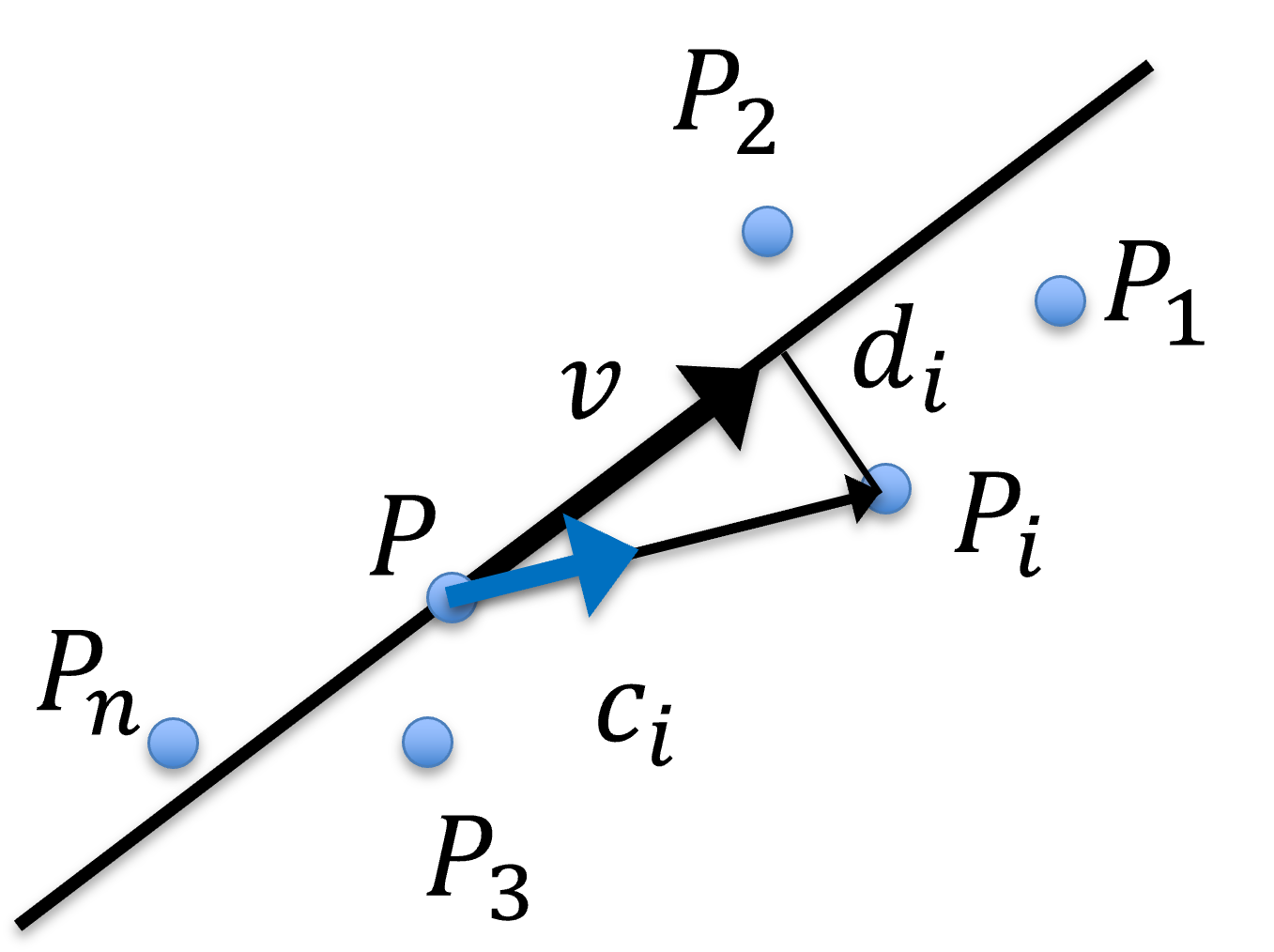
Figure 37:Fitting points to line in 3D, where are observed points, is the average, i.e. centre of gravity or centroid, of all , are the unit orientation vector from to each , and is the average of all .
The core concept for an easy solution is that, assuming the input data is decent in the sense that
there are sufficiently large number of observed points, and
there are little outliers, then the average is just as good as the least square minimum. This can be achieved by computing both an average point and an average orientation vector :
One should normalize all and flip them so they have the same genrral direction before computing .
As an optimization problem, the same precaution should be applied. One should always compute a set of error metric including but not limited to:
and set rules for outliers, such as
or
or and remove these outliers and recompute the optimization and error metrics. Repeat until no outlier is left or the input has been exausted.
Closed form solution via PCA
A closed form solution can be achieved using the Principal component analysis (PCA).
Thoughts on Averaging vs. Optimization
Optimization tend to yield better results than simple averaging,
Optimization are computationally more expensive than simple averaging,
Optimization (especially multi-variate non-linear ones) can be finicky, and they can be stuck in local minima and fail to accept acceptable results,
Most optimizations require an initialization (a guess serving as a starting point): most of the time an estimate such as averaging can serve as one,
If the input is decent, i.e. the cardinality of the dataset is sufficiently large and the cardinality of the outlier is relatively small (or you found a way to remove these outlier), the optimization may not improve much on the initial guess -- so you get by with simple averaging,
The good news is: for many least-square optimizations, such as fitting lines, planes, and quadratic surfaces, the optimum is guaranteed to exist and can be found without an initial guess,
Many of these fitting solutions exists on the internet,
Many closed-form solutions also exist, but they assume the absence of outliers!
- Al-Sharadqah, A., & Chernov, N. (2009). Error analysis for circle fitting algorithms. Electronic Journal of Statistics, 3, 886–911. 10.1214/09-EJS419