Now you understood an orthonormal basis can be defined by 3 observable points, and how the geometrical relationship between one cartesian coordinate system with another can be specified with a homogeneous transform. Now we present another method by means as an introduction to fiducial-based registration, bettern known as the Orthogonal Procrustes Analysis, or OPA.
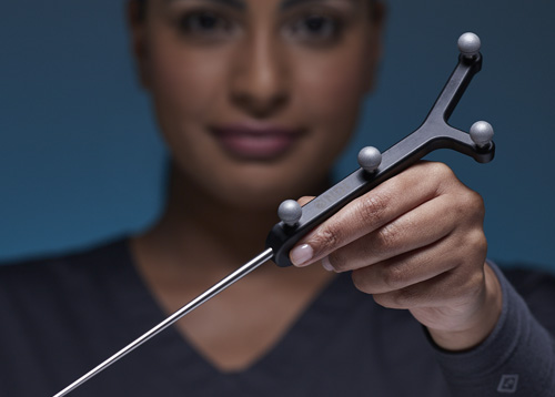
Figure 1:An optically-tracked stylus (probe) with 4 retro-reflective spheres. Image courtesy of Northen Digital Inc., accessed here, January 28, 2026.
From its dataset, you can see that a cartesian coordinate system was defined:
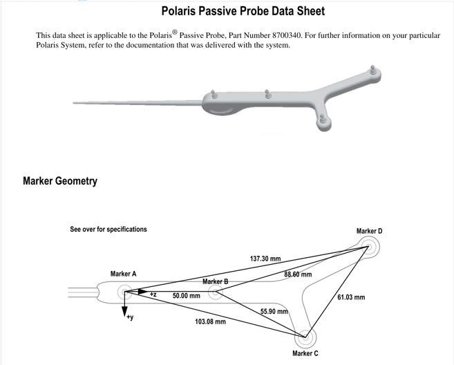
Figure 2:The marker geometry of an optically-tracked stylus (probe) with 4 retro-reflective spheres. Image courtesy of Northen Digital Inc., accessed on January 28, 2026.
where
Marker A is used as the origin,
Marker B is on the -axis,
Marker C is on the quadrant, and
Marker D is on the quadrant.
Each marker is bettern termed as a Fiducial: a point or a visible feature of an image used as a point of reference or a measure. Using the fiucial point as the origin and the fiducial point on the -axis , these four fiducial points are defined (or manufactured) as:
| Marker | x (mm) | y (mm) | z (mm) |
|---|---|---|---|
| A | 0.00 | 0.00 | 0.00 |
| B | 0.00 | 0.00 | 50.00 |
| C | 0.00 | 25.00 | 100.00 |
| D | 0.00 | -25.00 | 135.00 |
| tip | 10.00 | 0.00 | -150.00 |
Note that these points () are coplanar on the plane with . Let’s suppose that the tip of this stylus is located at .
While we have not learned about how a tracking system (spatial measurement device) work, assumes that each of these 4 fiducial points are observed by an optical tracking system via triangulation, and the coordinates of these 4 fiducial points in the home coordinate system of the optical tracker are:
| Marker | x (mm) | y (mm) | z (mm) |
|---|---|---|---|
| A | -39.00 | 59.00 | 33.00 |
| B | -39.00 | 10.0458 | 43.1728 |
| C | -51.6989 | -34.5271 | 74.4298 |
| D | -26.3011 | -77.5577 | 135.00 |
The question now is, where is the tip in the the coordinate system of the optical tracker?
Orthogonal Procrustes Analysis
To solve this problem, we must find the transform that represents the current position of these 4 fiducial points, and then apply the transform to the tip location. That is, we need to find the transform that maps the 4 marks that defined the cartesian coordinate system of the stylus (probe) to that of the optical tracker system:
and then apply the transform:
Given 2 sets of coordinates, this problem is commonly know as the Orthogonal Procrustes Analysis, a problem that spans many, many, scientific fields with solutions been invented and re-invented since the 1950’s. For engineering, both the solution based on SVD (Arun et al. (1987)) and unit quaternion (Horn (1987)) are commonly used and cited.
Below is an implementation to solve for the similarity transformation (i.e. with the possibility of isotropic scaling) that combines techniques from both:
function [R, t, a] = OPA( X, Y )
%
% INPUT:
%        X : matrix (3xn) 3D coordinates
%        Y : matrix (3xn) 3D coordinates
%
% OUTPUT:
%         solves the registration Y=R*a*X+t in least-square sense
%
%        R : 3x3 rotation
%        t : 3x1 translation
%        a : scalar scale
%
% Orthogonal Procrustes Problem, solving registration problem
% in the least-square sense
%
% Elvis C.S. Chen
% May 18, 2016
%
% minimal implementation

n = size(X,2); e = ones(n,1); II=eye(n)-((e*e')./n);
[U,S,V] = svd(Y*II*X');
R=U*[1 0 0; 0 1 0; 0 0 det(U*V')]*V';
% a = trace(S)/sum(sum((X*II).^2)); % from Schonemann 1970
% a = trace(S)/trace(X*II*X'); % from Schonemann 1970,alt
% a = trace(Y*II*Y')/trace((R'*Y)*II*X'); %from Fusiello 2015
a = sqrt( sum( sum((Y*II).^2) )/sum(sum((X*II).^2)) ); % from Horn 1987
% a = sqrt( trace( Y*II*Y' )/trace(X*II*X') );
t = mean( Y-R*a*X, 2);
Let see if this OPA code indeed work:
% generate a "random" transformation by generating 1) a rotation initiated
% by random numbers, and 2) a random 3x1 translation vector
Transform = eye(4)
Transform(1:3,1:3)=axang2rotm( rand(1,4) ); % rotation
Transform(1:3,4) = 100*rand(3,1) % translation

% n is number of fiducial points
n = 4;
ModelPoints = 50 * rand(3,n);
ModelPoints(4,:) = ones(1,n); % append 1 for homogeneous coordinate

% MeasuredPoints are the transformed points
MeasuredPoints = Transform * ModelPoints;

% Question is: given the ModelPoints and MeasuredPoints,
% can we recover the transformation?

[R,t,a] = OPA(ModelPoints(1:3,:), MeasuredPoints(1:3,:))
Try the code yourself, and determine if the output of the OPA code (R for rotation and t for translation) correspond to the random transformation you just generated.
The Matlab code above serve as an example for you to compute the location of the stylus tip in the tracking system for the example above.
- Arun, K. S., Huang, T. S., & Blostein, S. D. (1987). Least-Squares Fitting of Two 3-D Point Sets. IEEE Transactions on Pattern Analysis and Machine Intelligence, PAMI-9(5), 698–700. 10.1109/TPAMI.1987.4767965
- Horn, B. K. P. (1987). Closed-form solution of absolute orientation using unit quaternions. Journal of the Optical Society of America A, 4(4), 629–642. 10.1364/JOSAA.4.000629