In linear algebra, transform (or transformation matrix) is used to specify the geometrical relationship between two cartesian coordinate system. There are many use cases:
Co-registration between CT and {term}`MRI> volumes
Specify the 3D location of an object using tracking systems,
Tool calibration, e.g. specifying the location of the tip of surgical drill with respect to the tracking sensor, etc.
That is, in an IGI surgical workflow, there are always multiple rigid bodies, i.e. cartesian coordinate system present:
Target anatomy (spine),
Surgical tool (needle),
Live image or video US) and
Geometrical model or representation of anatomy (e.g. surface model derived from CT)
We must keep track of them all the time by understanding how each of these cartesian coordinate system are related with each other.
Translation
The simplest transform is moving a object from one location to another, i.e. a translation.
Let the initial position of an object be , and let be a translation vector, then the new position of the object after translation by is:
If both and are multi-dimensional, then this is equivalant to vector addition. In 3D, we have $$
$$
In Python, we can simply use the standard addition operation:
import math
import numpy as np
import numpy.matlib

p = np.array([ 1, 0, 0 ])      # This is a ROW vector
p = p.reshape(-1, 1)           # this is a COLUMN vector
p = np.array([ [0],[1],[0] ])  # alternative

v = np.array( [4, 5, 6] ).reshape(-1,1)
q = p + v

print("The initial position is:\n", p,
"\nafter translation by:\n", v,
"\nis now located at:\n", q)
The initial position is:
[[0]
[1]
[0]]
after translation by:
[[4]
[5]
[6]]
is now located at:
[[4]
[6]
[6]]
For visualization and other implementations, consult the following tutorial.
Rotation
In 3D, rotation is specified as matrix , and using colomn vector, a point is rotated by into as:
Rigid Rotation
We are particularly interested in rigid rotation, that that simply rotates an object but do not change its geometry (length, volumen, etc.,). For a matrix to be a rigid rotation, the following properties must be satisfied:
Each row and each column is a unit vector,
The dot product between each row with every other is 0.
In other word, a rigid rotation is akin to set up an orthonormal axes: each axis has a unit length one, and each axis is perpendicular with each other.
One consequence of these two properties is:
The determinant of a rigid rotation is 1.
Let’s look at some examples.
Rotation about z-axis
Perhaps the most familiar rotation is in fact the rotation about the -axis. Most of us are used to perform or study rotation in 2D, i.e. the x-y plane, which is in fact equivalent to rotation about the -axis.
The rotation is performed about an axis, called the axis of rotation, by an angle . Using the RHR, and when looking from the positive towards the negative of the axis of rotation, the CCW rotation is the positive angle.
That is, if the right-thumb points to the positive direction of the axis of rotation, then the curve of the fingers is the positive rotation.
It should be noted that a point on the axis of rotation is invariant under rotation.
Let’s visualize this: suppose a point and is located on the - and -axis, respective, and after rotation, we have
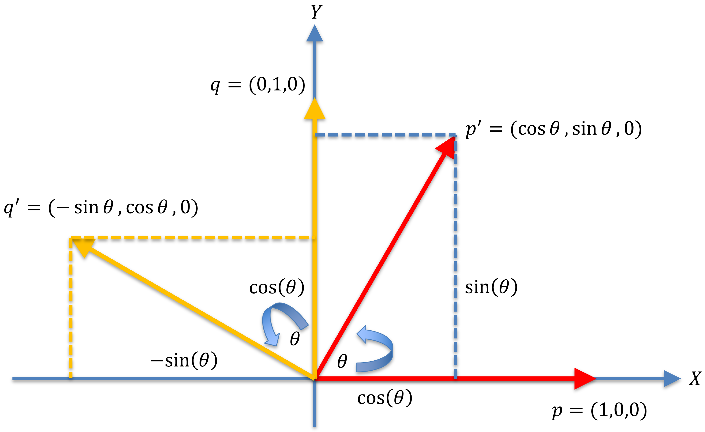
Figure 1:Rotation about -axis visualized.
And for any point on the -axis, rotation about the -axis does not move :
It can be implemented in Python as:
import numpy as np
import math

def rotZ3x3( angle_rad ):
    # return a 3x3 rotation about z-axis, where angle is specified in radian

    c = math.cos( angle_rad )
    s = math.sin( angle_rad )
    # a 3x3 identity matrix
    R = np.identity(3)

    # specify the elements of the rotation
    R[0,0] =  c
    R[0,1] = -s
    R[1,0] =  s
    R[1,1] =  c
    return R
A simple test:
p = np.array([1,0,0]).reshape(-1,1)

# rotation by 90 degree
print( np.around( np.matmul( rotZ3x3( math.pi/2 ) , p) ) )
# print( rotZ3x3( math.pi/2 )@p )  # short cut, the @ sign is matrix multiplication
[[0.]
[1.]
[0.]]
Suppose you rotate an object by an angle , and immediately rotate it by an angle : nothing changes. Is it true numerically?
You should also notice that , the transpose.
# rotation by pi/4 followed by rotation by -pi/4
print( np.around( np.matmul( rotZ3x3( -math.pi/4 ) , rotZ3x3( math.pi/4)) ) )
[[1. 0. 0.]
[0. 1. 0.]
[0. 0. 1.]]
Rotation about -axis
To visualize how to perform rotation about the -axis, position yourself at direction looking towards the origin.
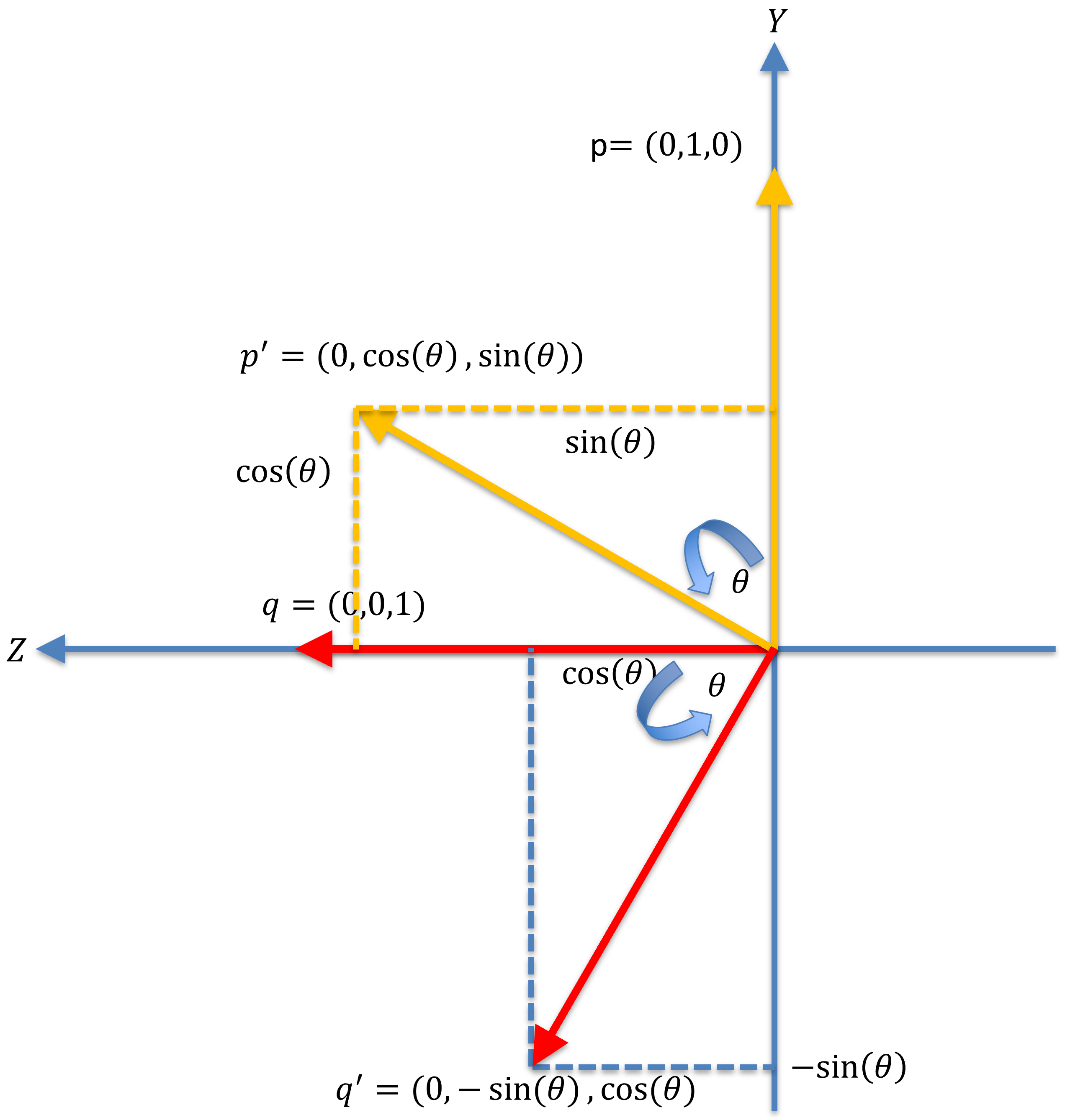
Figure 2:Rotation about -axis visualized.
Again, a point on the -axis remains invariant under rotation about the -axis.
Using this visualization, one can infer that the rotation about the -axis by an angle is:
def rotX3x3( angle_rad ):
    # return a 3x3 rotation about z-axis, where angle is specified in radian

    c = math.cos( angle_rad )
    s = math.sin( angle_rad )
    # a 3x3 identity matrix
    R = np.identity(3)

    # specify the elements of the rotation
    R[1,1] =  c
    R[1,2] = -s
    R[2,1] =  s
    R[2,2] =  c
    return R
[[ 1. 0. 0.]
[ 0. 0. -1.]
[ 0. 1. 0.]]
Rotation about -axis
To visualize how to perform rotation about the -axis, position yourself at direction looking towards the origin.
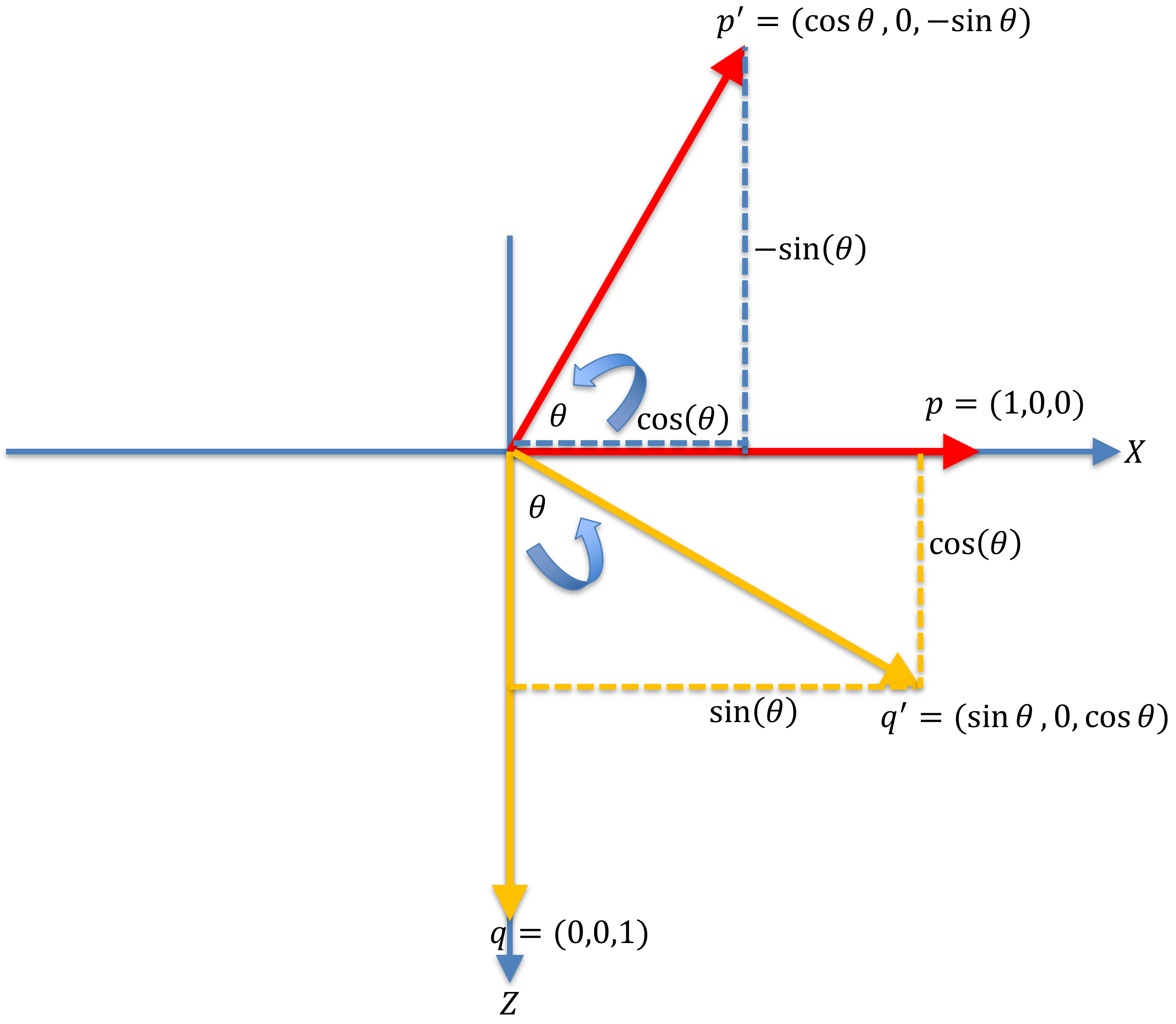
Figure 3:Rotation about -axis visualized.
Again, a point on the -axis remains invariant under rotation about the -axis.
Using this visualization, one can infer that the rotation about the -axis by an angle is:
def rotY3x3( angle_rad ):
# return a 3x3 rotation about z-axis, where angle is specified in radian
c = math.cos( angle_rad )
s = math.sin( angle_rad )
# a 3x3 identity matrix
R = np.identity(3)
# specify the elements of the rotation
R[0,0] = c
R[0,2] = s
R[2,0] = -s
R[2,2] = c
return RSuccessive Rotations
Suppose you are interested in rotating an object about the -axis by an angle , and further by rotating the rotated object about the -axis by an angle , how would this be achieved?
Let be the rotated object after the rotation about the -axis by an angle :
and be the rotated object after the rotation about the -axis by an angle :
Thus
Because matrix multiplication is associative, we can indeed define a combined rotation matrix:
and
That is, instead of thinking about successive rotations as a series of rotations, it is often more intuitive to think of it as just one rotation about an axis of rotation instead.
For visualization and other implementations, consult the following tutorial.
Rotation About an Unit Vector
One omission in the above introduction to rotation, one is often done, is that rotation is performed about a vector. In the previous examples, i.e. rotation about -, -, and -axis, is in fact rotation about the orthonormal basis located at the origin.
That is, rotation about the -axis should been seen as rotation about the unit originated at
In fact, the rotation can be perform about an arbitrary axis in space. The axis of rotation is specified as a unit orientation vector anchord at a point .
If the axis of rotation is originated at the origin , than rotation about the unit vector by an angle can be represented as a rotation matrix using the following formula:
def axang2rotm( anang ):
#
# Convert the axis-angle rotation into a 3x3 rotation matrix
#
# The name is the same as the equivalent function in Matlab (under Navigation Toolbox)
#
# Assumes that axang is a row vector of 4:
#
# axanx = numpy.array([vx, vy, vz, angle])
#
# where (vx,vy,vz) is axis of rotation, and
# angle in radian
#
# extract components from the input vector
x = anang[0]
y = anang[1]
z = anang[2]
angle = anang[3]
# make sure that and axis of rotation is a unit vector
l = math.sqrt(x*x + y*y + z*z)
x = x/l
y = y/l
z = z/l
R = np.identity(3)
xx = x * x
xy = x * y
xz = x * z
yy = y * y
yz = y * z
zz = z * z
ca = math.cos( angle )
sa = math.sin( angle )
vers_a = 1 - ca # versine(angle) = 2 * sin^2(angle/2)
R[0,0] = xx * vers_a + ca
R[0,1] = xy * vers_a - z * sa
R[0,2] = xz * vers_a + y * sa
R[1,0] = xy * vers_a + z * sa
R[1,1] = yy * vers_a + ca
R[1,2] = yz * vers_a - x * sa
R[2,0] = xz * vers_a - y * sa
R[2,1] = yz * vers_a + x * sa
R[2,2] = zz * vers_a + ca
return RYou can verify if we can use the above function to reproduce rotation about -, -, and -axis:
print( "rotation about x-axis by 90 degree is:\n", np.around(axang2rotm(np.array([1,0,0,math.pi/2]))))
print( "rotation about y-axis by 90 degree is:\n", np.around(axang2rotm(np.array([0,1,0,math.pi/2]))))
print( "rotation about z-axis by 90 degree is:\n", np.around(axang2rotm(np.array([0,0,1,math.pi/2]))))rotation about x-axis by 90 degree is:
[[ 1.  0.  0.]
 [ 0.  0. -1.]
 [ 0.  1.  0.]]
rotation about y-axis by 90 degree is:
[[ 0. 0. 1.]
[ 0. 1. 0.]
[-1. 0. 0.]]
rotation about z-axis by 90 degree is:
[[ 0. -1. 0.]
[ 1. 0. 0.]
[ 0. 0. 1.]]
We can verify our formulation against vtkTransform
import math
import numpy as np

from vtkmodules.vtkCommonTransforms import vtkTransform
myTransform = vtkTransform()
myTransform.PostMultiply()
myTransform.Identity()
myTransform.RotateWXYZ( 33, 1, 2, 3) # angle in degree
print("Our implementation: \n", axang2rotm(np.array([1,2,3,33*math.pi/180])), "\n")
print("VTK implementation: \n", myTransform.GetMatrix())Our implementation:
[[ 0.8501941 -0.41363565 0.3256924 ]
[ 0.45972978 0.88476469 -0.07641972]
[-0.25655122 0.21470209 0.94238235]]
VTK implementation:
vtkMatrix4x4 (000002829DD518B0)
Debug: Off
Modified Time: 84
Reference Count: 2
Registered Events: (none)
Elements:
0.850194 -0.413636 0.325692 0
0.45973 0.884765 -0.0764197 0
-0.256551 0.214702 0.942382 0
0 0 0 1
What If the Axis of Rotation does not Originate from the Origin?
If the axis of rotation does not originate from the origin, i.e. for any and a fixed point on the line, then rotation about by an angle is performe in 3 steps:
Translate by , i.e. so now the rotation is performed about that is originated from the origin ,
Perform rotation about by , followed by
Translate by
Homogeneous Transformation
Suppower you want to rotate an object (e.g. a point) about a vector that does not originate from the origin (i.e. ), base on this discussion you would need to perform the following operation in succession:
Translate by , i.e.
Rotate by by , i.e.
Translate by , i.e.
which involves column vectors (translation) and square matrices (rotation), with two operators (vectors addition and matrix multiplication). For a longer, successive operations of translations and rotation, both the notation and mathematical operation will become intractable very quickly.
The solution is to work in homogeneous coordinates instead. That is, instead of using matrix and vector to represent rotation and translation, respectively, one use matrix to represent both.
For example, rotation about -axis by an angle is now represented as:
Rotation about -axis by an angle is:
Rotation about -axis by an angle is:
Successive Transforms
Notice that both translation and rotation are now represented as matrices. Apply either the translation or the rotation operation is now performed as matrix multiplication. To translate a point by , append a 1 as the column:
and after matrix multiplication:
which is same as before.
Successive transformations such as rotation about an arbitrary vector is now represented as matrices multiplication:
Moreover, the inverse transform can be trivially found by computing the inverse of the matrices. This left as an exercise for you. You may wish to consult this old but concise document for detail.
For visualization and other implementations, consult the following tutorial.
Change of Persectives
Suppose Alice and Bob are sitting on a couch watching TV. The TV is directly in front of Alice, and Bob sits on the right of Alice. Where is the TV from Bob’s perspective?
For the purpose of the discussion, let the COG of the TV denotes the position of the TV. If we assign a cartesian coordinate system to Bob, we can specify a coordinate the location of the TV from Bob’s perspective. For this trivial example, suppose the TV is located at at the coordinate system associated with Bob
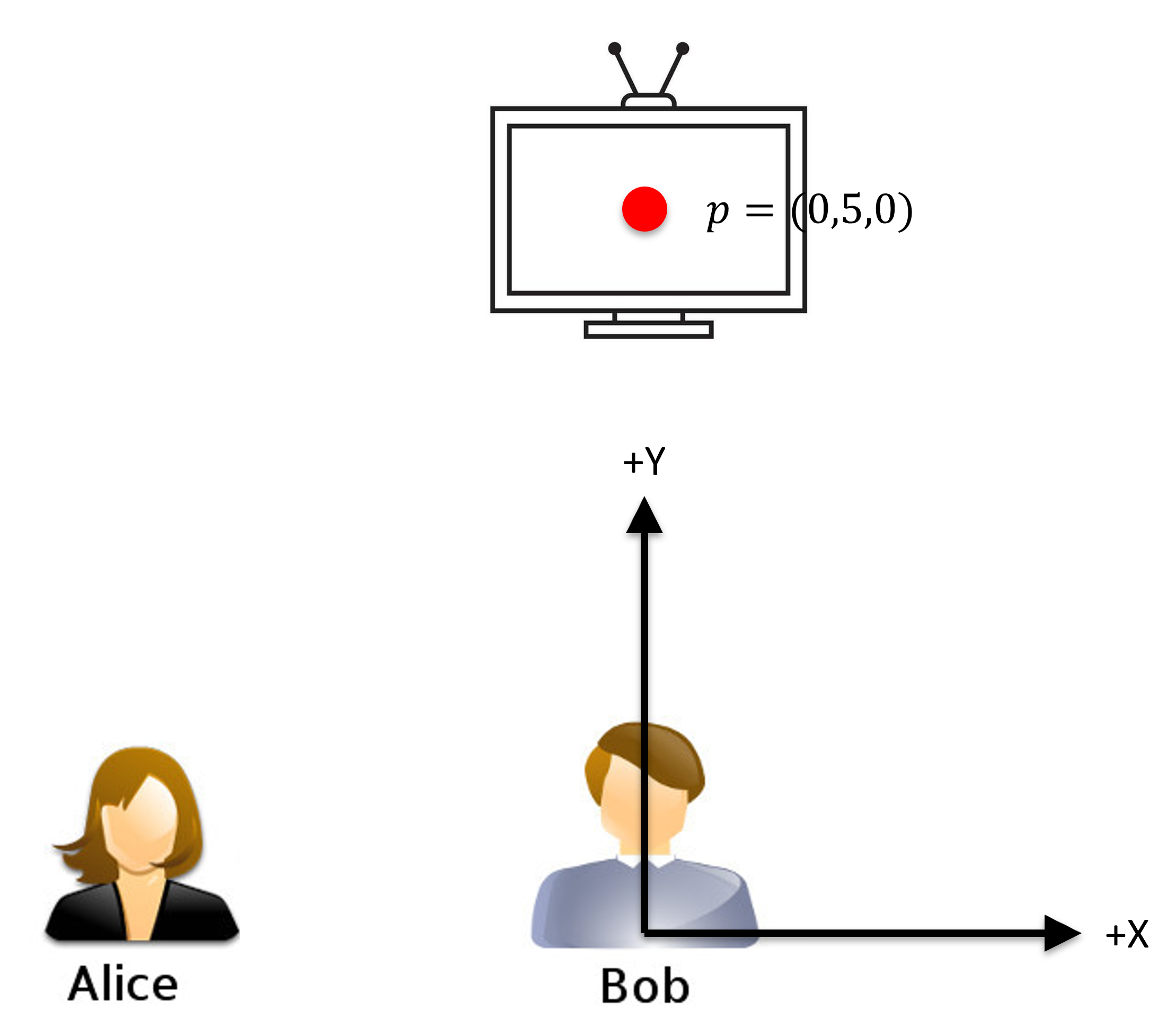
Figure 4:The position, denoted as a red circle, is specified from Bob’s perspective.
Suppose Alice is sitting sitting at (from Bob’s perspective). We can also assign a cartesian coordinate system to Alice: for the moment, assume that the orientation of Alice’s and Bob’s cartesian coordinate system have the same orientation. That is, both of their -axis point to the same direction, and both their -axis point to the same direction.
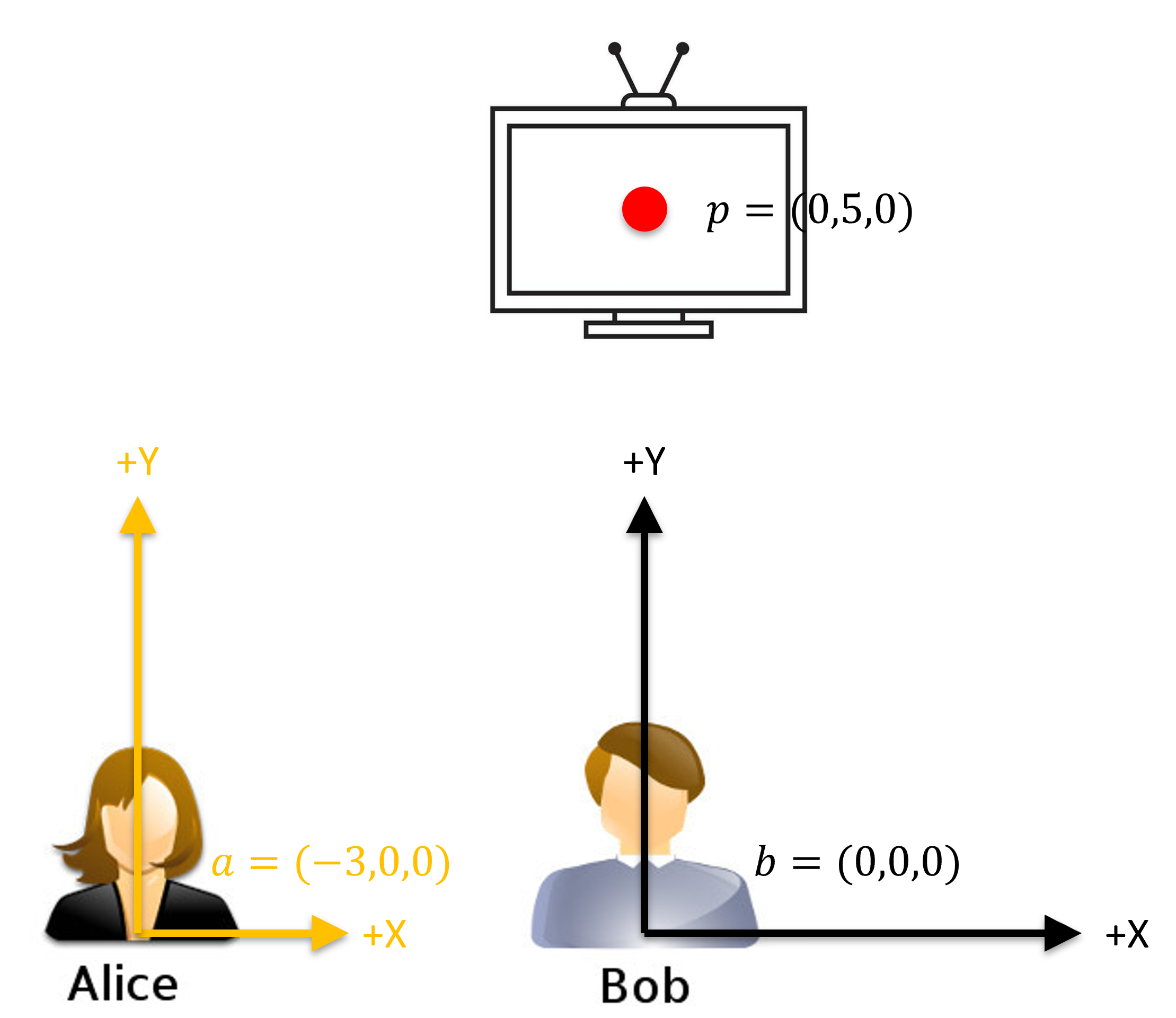
Figure 5:Alice sits next to Bob.
Where is the TV () from Alice’s perspective?
From Figure 5 you may infer that, because Bob is at (i.e. inverse of where Alice is from Bob), and the TV is located at from Bob, the TV is located at from Alice.
But how do we express this mathematically?
Transformation: Translation
Let denote the geometrical relationship between Alice and Bob from Bob’s perspective:
We adopt the notation of and to indicate the transformation one coordinate system to . For example, the location of Alice, , in her local coordinate system can be brought from to via:
Conversely, from Alice’s point of view, Bob is located at , and
Notice that is the inverse of (You should verify this by computing the inverse of the matrices themselves). Notice that the position of the TV is from Bob’s perspective, we can compute where it is from Alice’s perspective using the transformation:
One Key to help you in writing down this sequence os matrix multiplication is to note that the successive and must match.
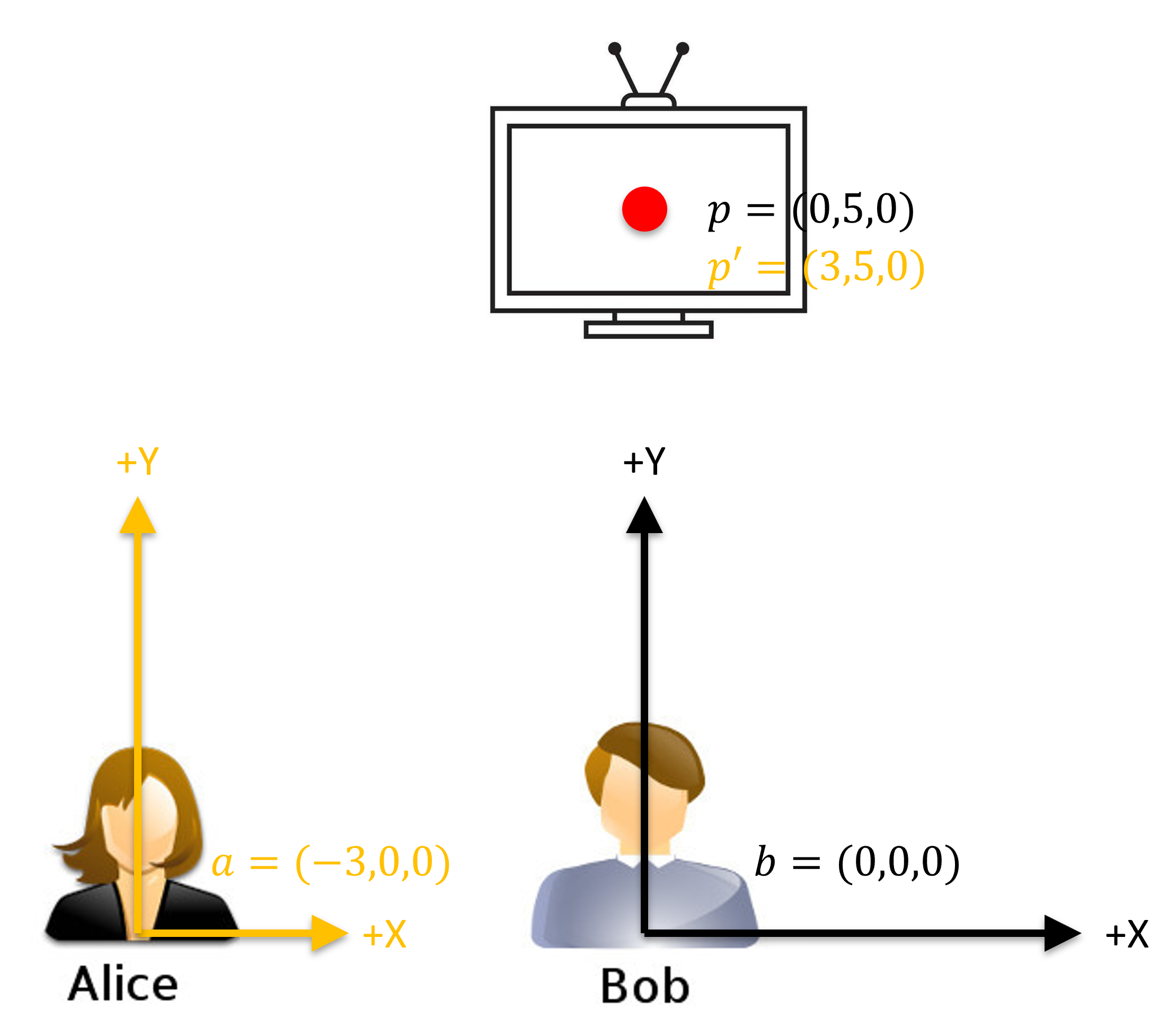
Figure 6:Location of TV from Alice’s perspective.
To illustrate this point one more time, now we know that the TV, from Alice’s perspective, is located at . To find out where it is from Bob’s perspective, we use:
Transformation: Rotation and Translation
In the previous discussion, the transform only involves a simple translation (between Alice and Bob). What if Alice defines her local coordinate system differently than Bob (say, she’s left handed and Bob is right handed?).
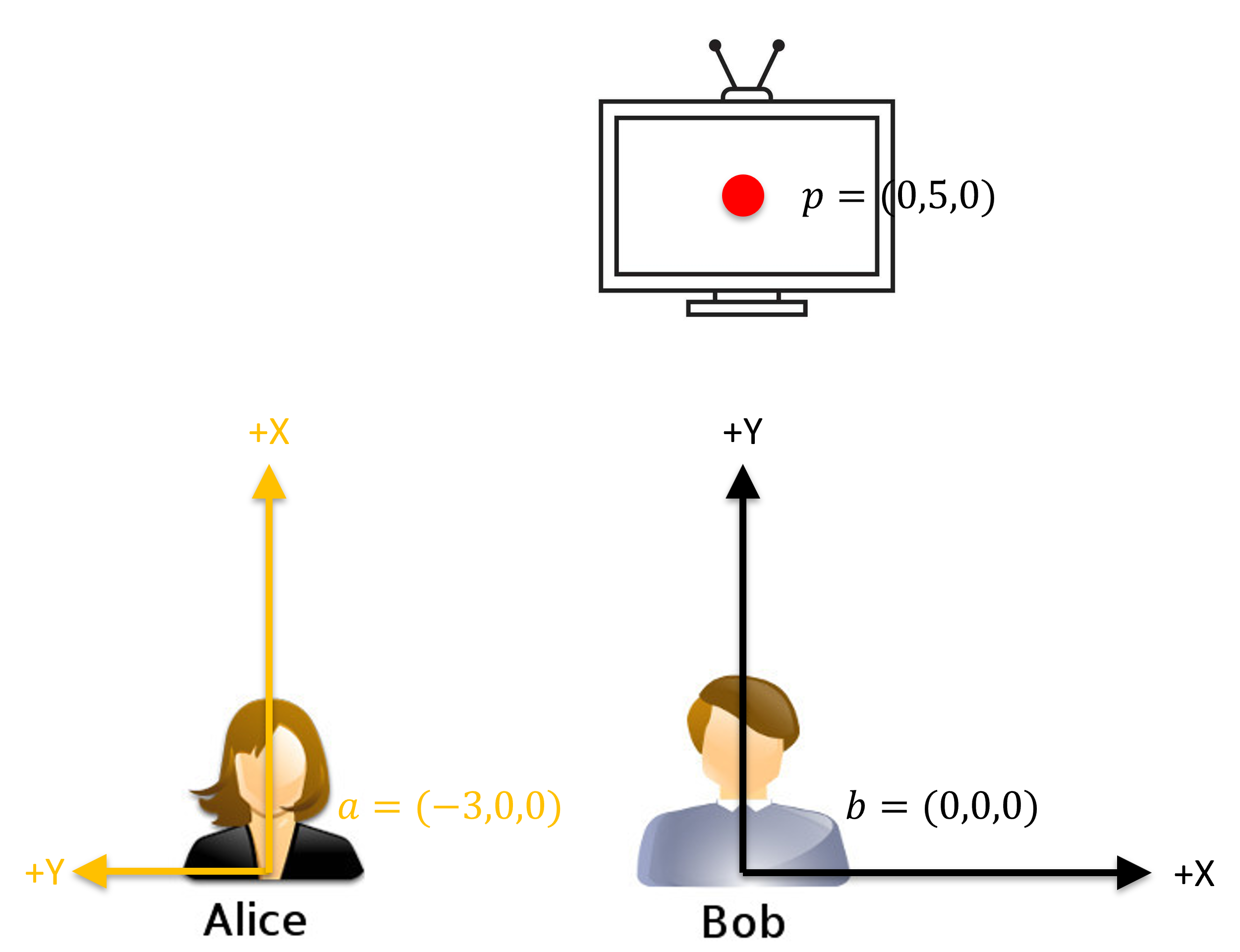
Figure 7:The orientation of the local coordinate system of Alice is different than that of Bob.
You will notice that there is a rotation about the -axis by between Alice’s and Bob’s coordinate systems:
and
And in this new coordinate system of Alice, the location of the TV is now:
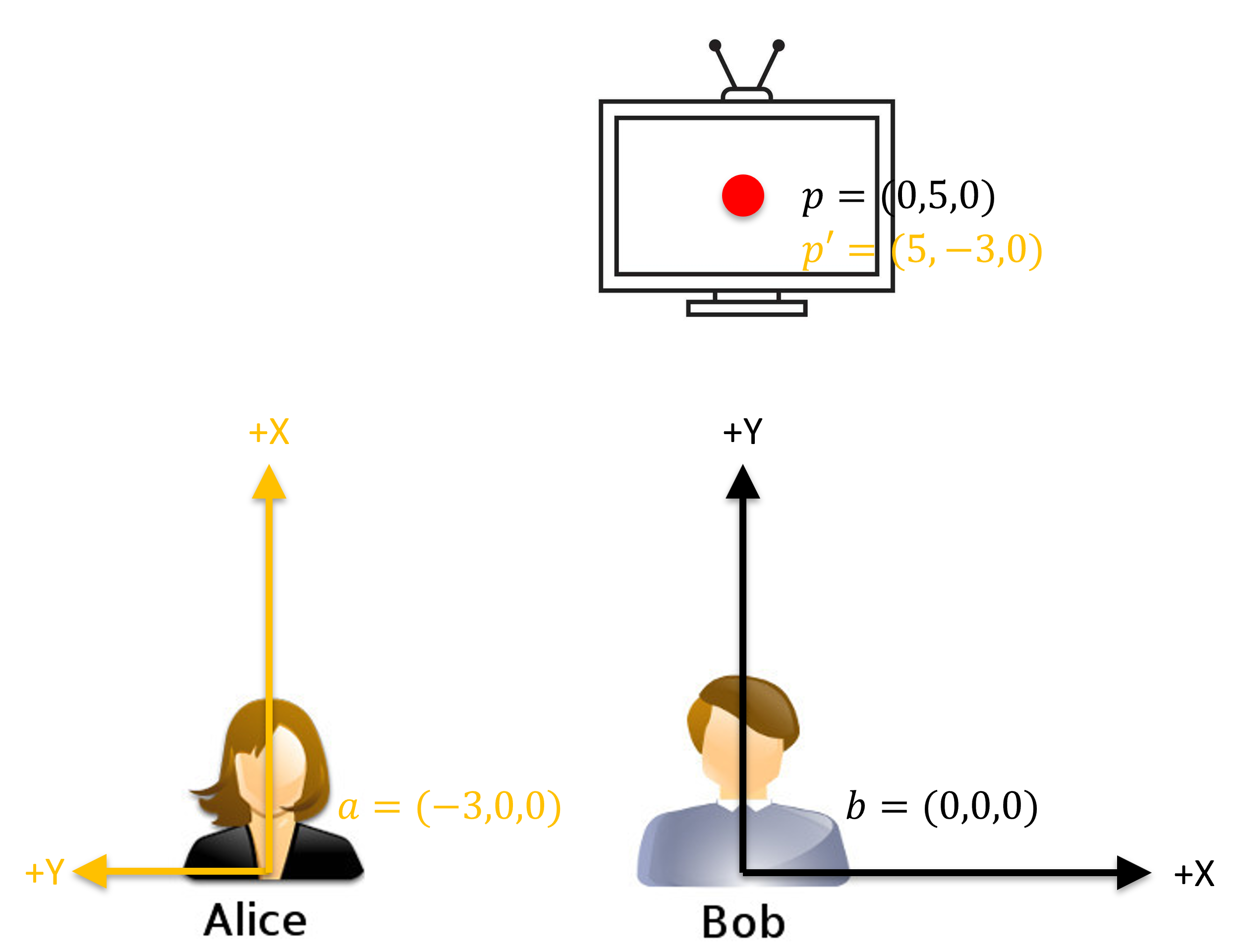
Figure 8:The coordinate of the TV from Alice’s perspective.
But How?
To walk you through the process of constructing the transform that links one coordinate system with another, refer to Figure 8. To construct the transformation that see what Alice sees from Bob’s perspective, consider
How are the base vectors of Alice’s coordinate system mapped to Bob’s, and
How is the origin of Alice’s coordinate system mapped to Bob’s.
We proceed by noticing that
The -axis of Alice’s coordinate system, which maps to Bob’s -axis ( colume of ),
The -axis of Alice’s coordinate system, which maps to Bob’s -axis ( colume of ),
The -axis of Alice’s coordinate system, which maps to Bob’s -axis ( colume of , i.e. no change), and
The origin of Alice’s coordinate system is located at from Bob’s point of view ( column of ).
That is,
The rotational component of the transformation is to map the base axes from one another, and
The translational component of the transformation is the translation of the origins.